Project 4: Image Warping and Mosaicing
Part 4A
Part 1.1: Shoot the Pictures
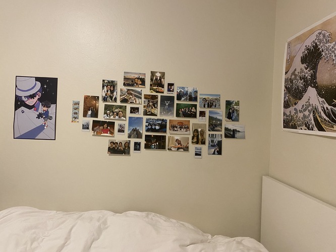
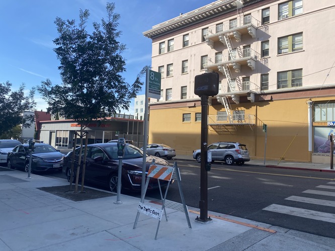
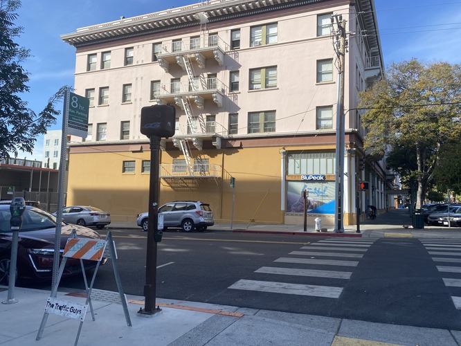
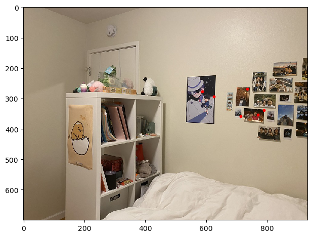
These are the pictures I took of Brown's by the College of Natural Resources, my room, and the intersection outside of Identity. I made sure to adjust only the angle at which the camera was facing and kept the position of my camera the same as I shot, to ensure that I maintained the same center of projection. I tried to aim for an approximate 40-70% overlap and ensure minimal moving objects.
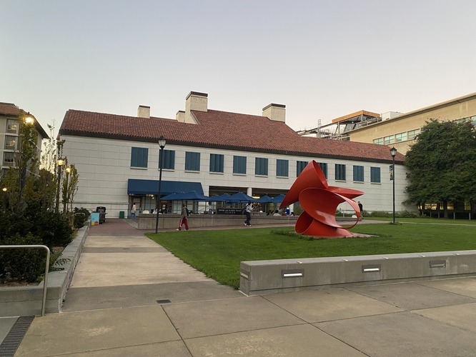
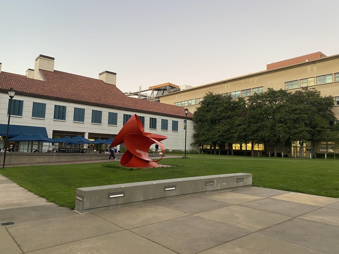
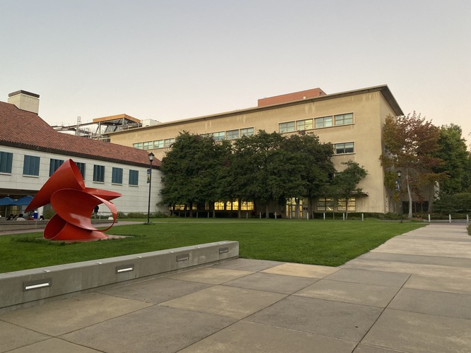
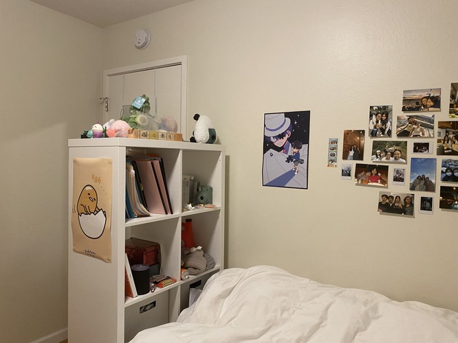
Part 1.2: Recover Homographies
Next, I needed to compute homographies by writing a computeH function. This transformation follows the format p' = Hp, where H is a 3x3 matrix with 8 degrees of freedom, which we are looking for. To do this, I worked through the following computation:
Which I then simplified to the general form by reorganizing the above equation and isolating the a through h variables into a single vector into the form \( A = xB \): $$ \begin{bmatrix} px & py & 1 & 0 & 0 & 0 & -px \cdot qx & -py \cdot qx \\ 0 & 0 & 0 & px & py & 1 & -px \cdot qy & -py \cdot qy \end{bmatrix} \cdot \begin{bmatrix} a \\ b \\ c \\ d \\ e \\ f \\ g \\ h \end{bmatrix} = \begin{bmatrix} qx \\ qy \end{bmatrix} $$
Now, I can perform a basic matrix multiplication to solve for my 8 unknowns. To do this, I created the left and right matrices A and B and extended it for every point in the left image (px, py) and its corresponding point (qx, qy) in the right image. This creates an overdetermined system which I solved for by leveraging the least squares formula \( x = (A^T A)^{-1} A^T B \), ultimately allowing me to retrieve my 8 unknowns and populate these into a homography matrix H.
Part 1.3: Warp the Images
For image warping, I defined a function warpImage(im, H) that applies the homography H created from computeH and applies it to image im. My goal is to transform my first image im such that it aligns with my reference image.
First, I did this by finding the corner points of my image, transforming them, and also shifting them such that they are in the positive coordinate space. Then, after performing the same shift to my reference image, I can compute my homography matrix H which will map my first image to my reference image such that its correspondence points line up perfectly.
From there, I create a new, blank image of a polygon shape using sk.draw.polygon with my shifted corner points. I then inverse warped these polygon pixels to the original first image's positions, and then copied these pixels over to my new image by working with each rgb channel individually.
I have 3 CNR images (left, middle, and right) that I defined correspondence points for between the left and middle images, as well as the middle and right images. Using my middle image as the reference, I computed homographies for the left and right images onto my middle image and made sure all alignment and shifting was correct.


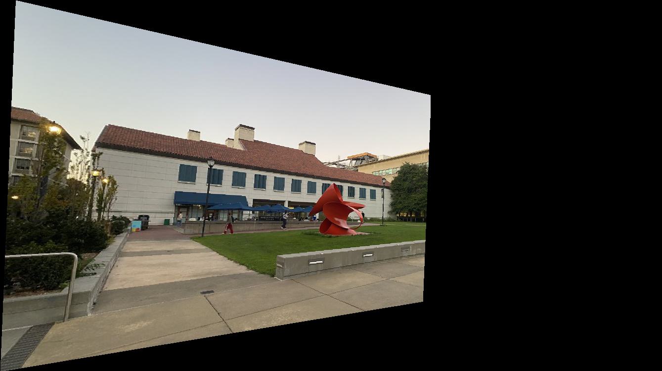
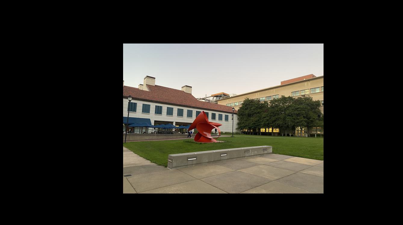
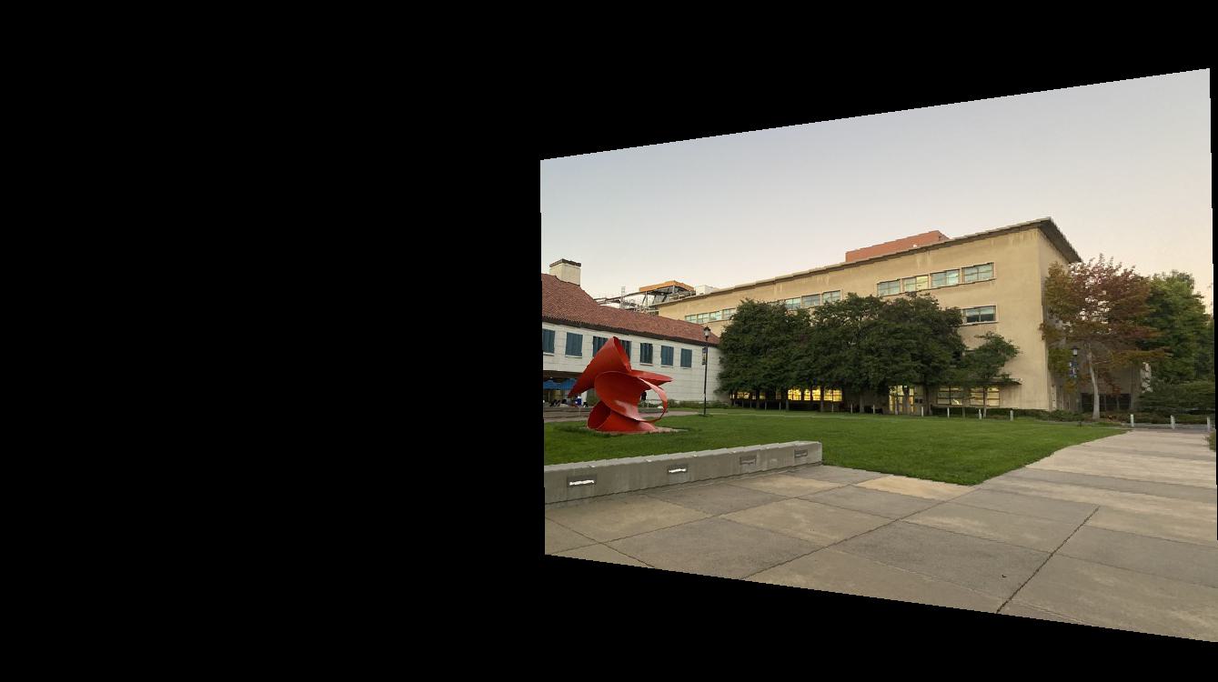
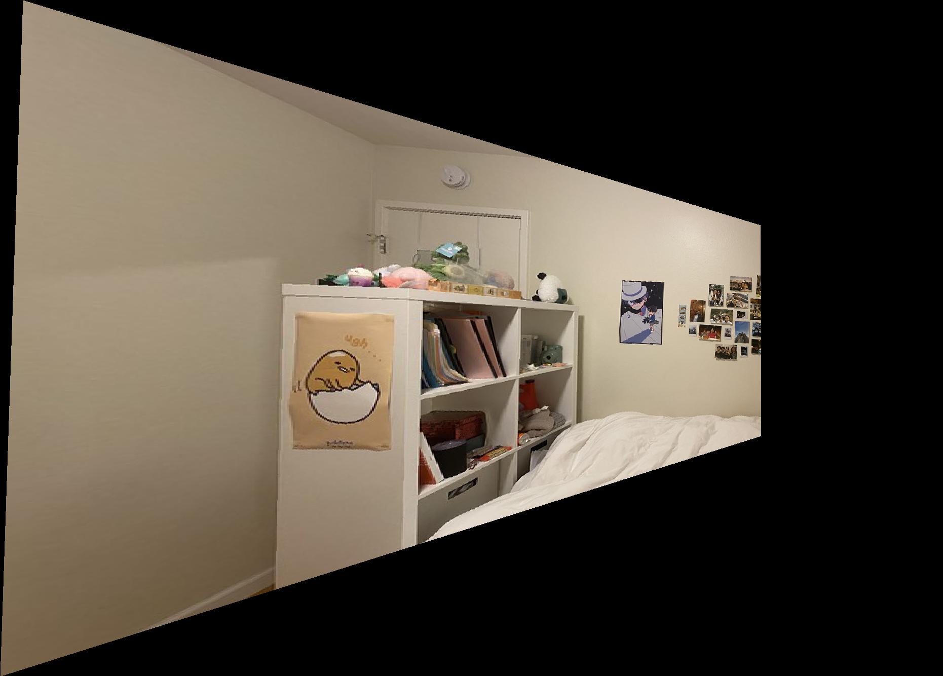
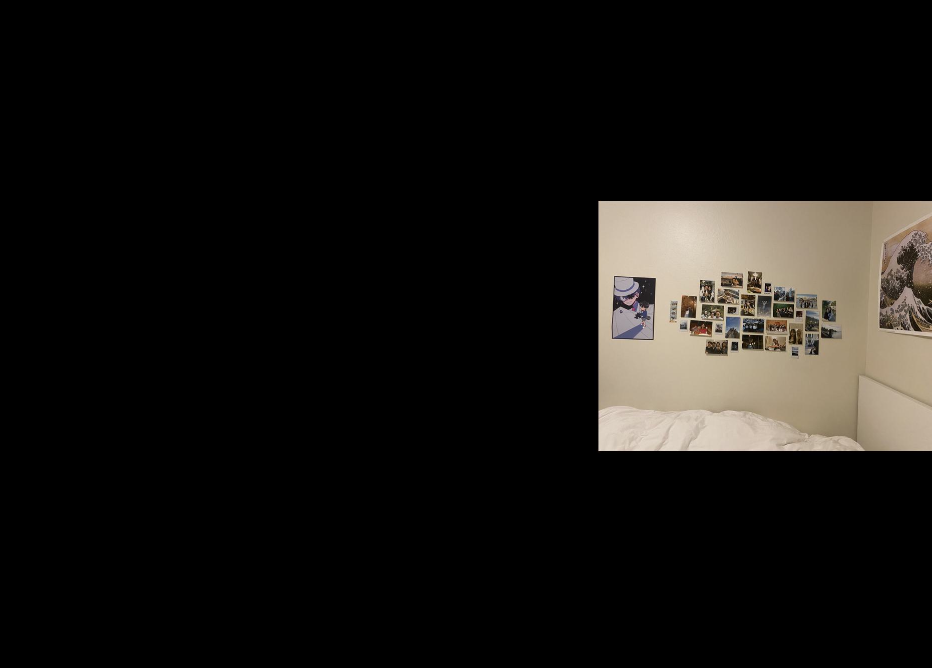
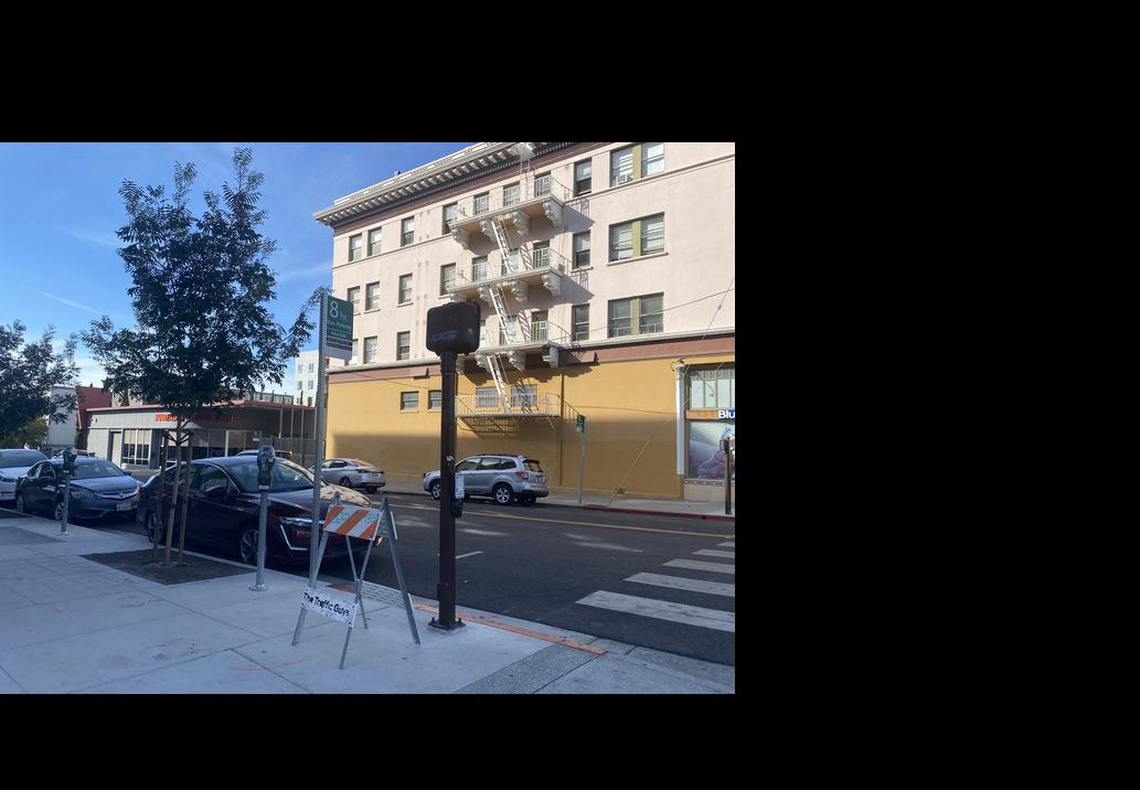
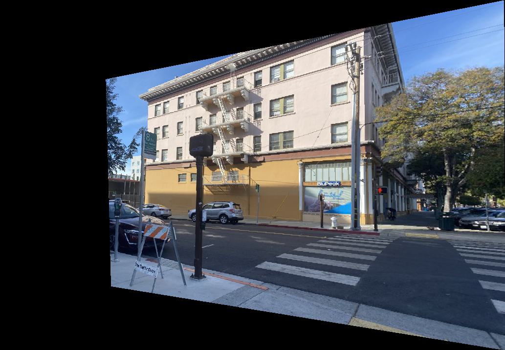
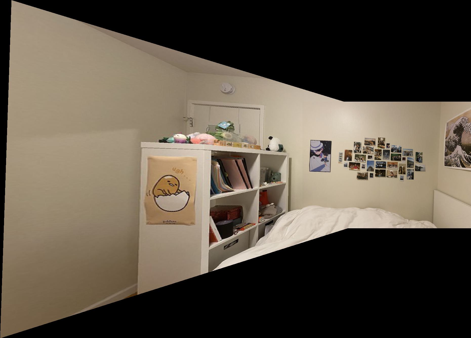
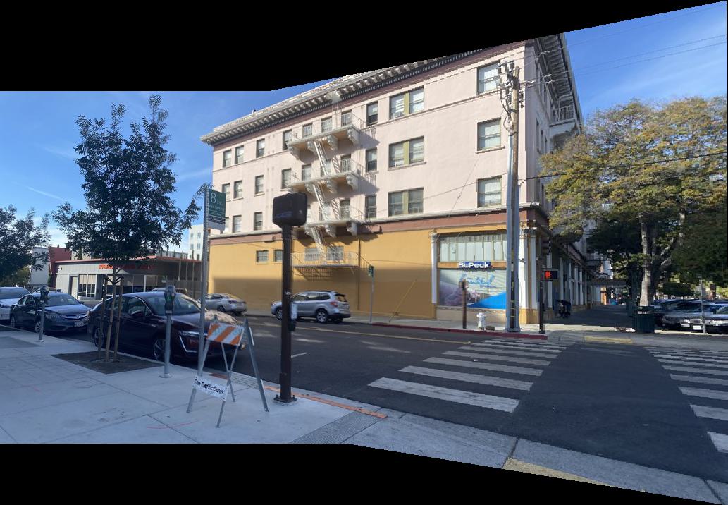
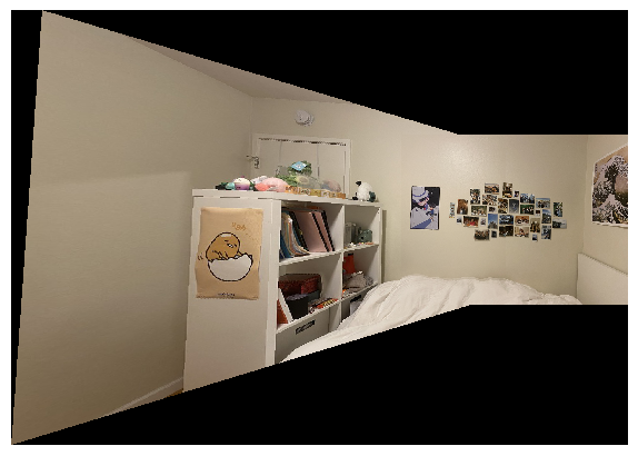
For the other two sets of images, I wanted to try warping one onto the other. For my room, I warped my left image onto my right image, and for Identity, I warped my right image onto my left image as so:




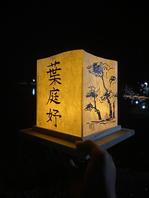
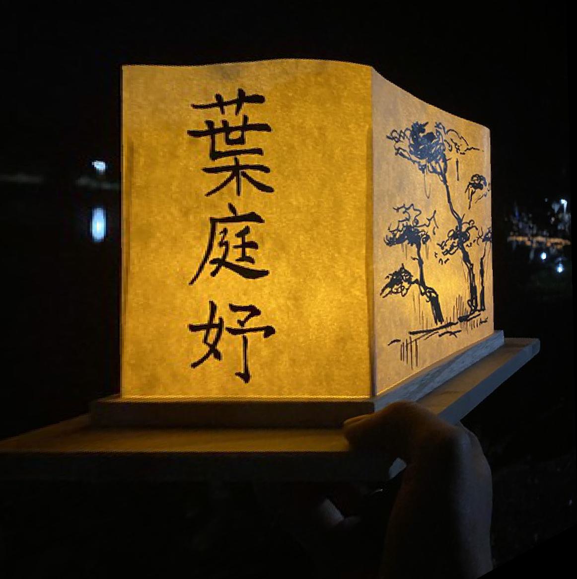
Part 1.4: Image Rectification
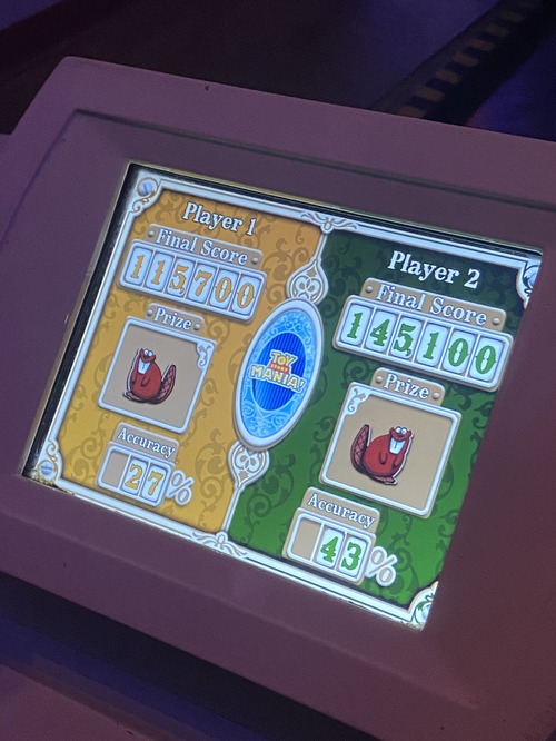
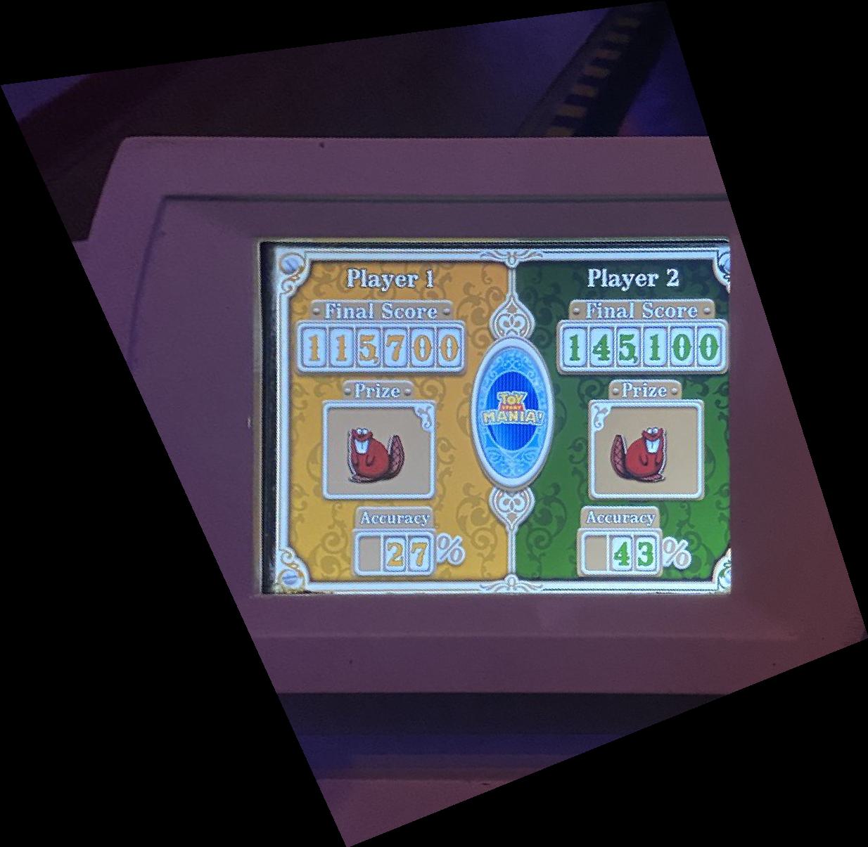
For image rectification, I am confirming the accuracy of my homography computation by
taking a square or rectangular surface taken at an angle, transforming using homography,
and then producing a warped image such that it is rectangular and looks "flat" from the
viewer's point of view. I used corner correspondence points of the object as well as
hardcoded corner points [[0, 1], [1, 1], [1, 0], [0, 0]] that are scaled to the image.
Provided are an examples of my angled images which I made rectangular using a homographic
transformation.
Part 1.5: Blend the images into a mosaic
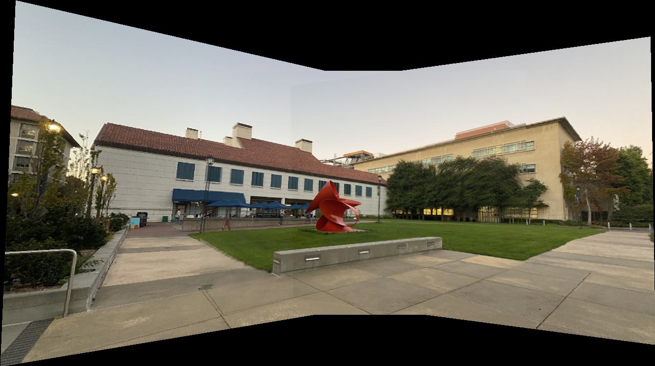
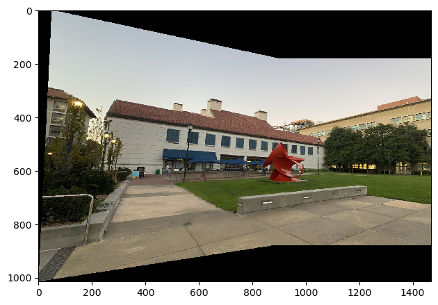
Finally, with my computeH and wrapImage function, I am equipped to warp my images together to produce a combined image with information from all input images. For my 3 CNR images, I will warp my left and right images onto the middle one.


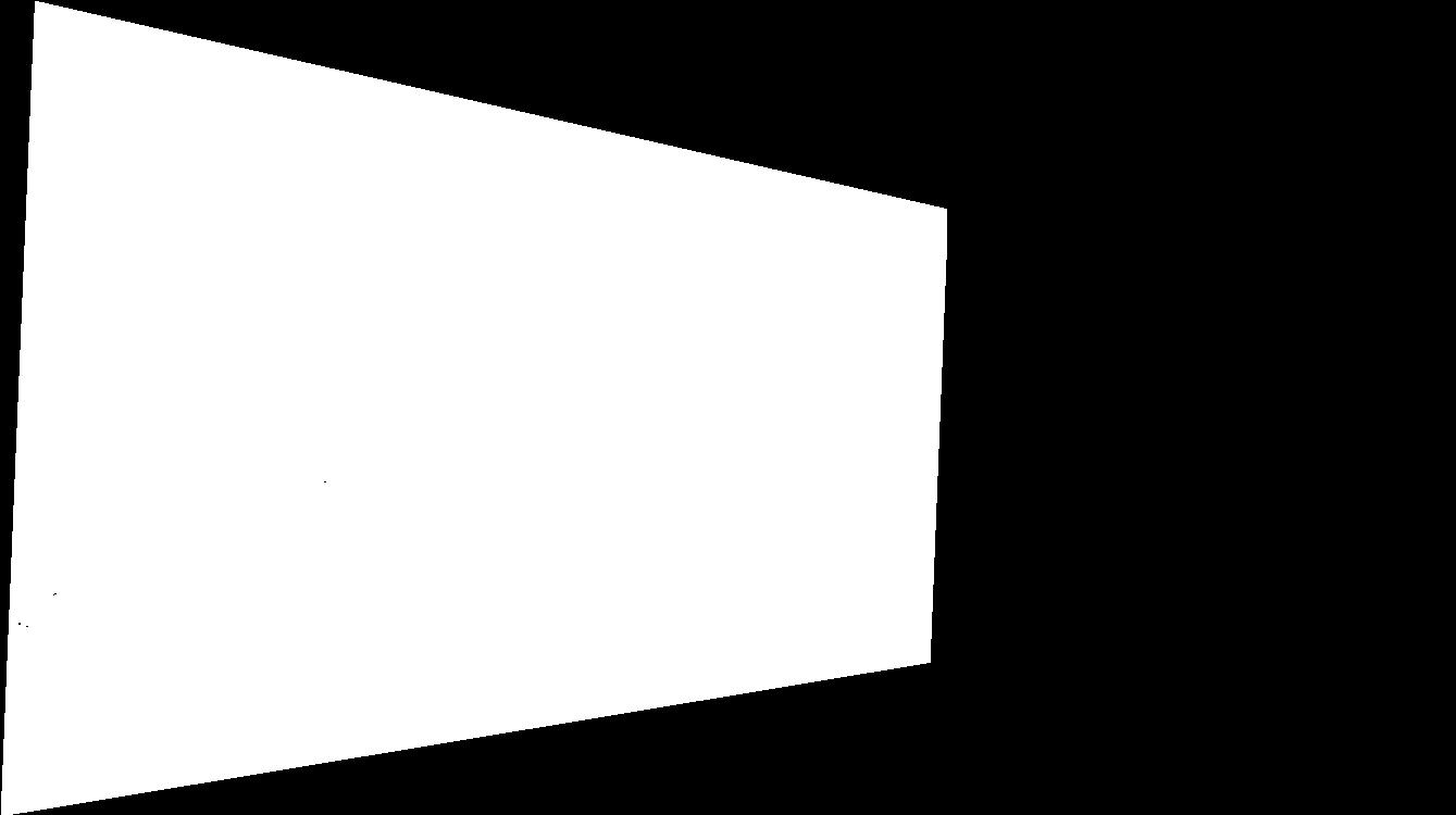
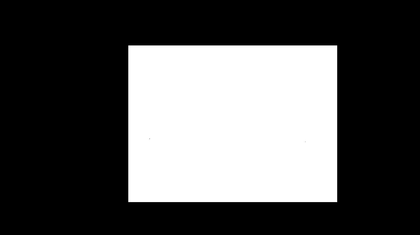
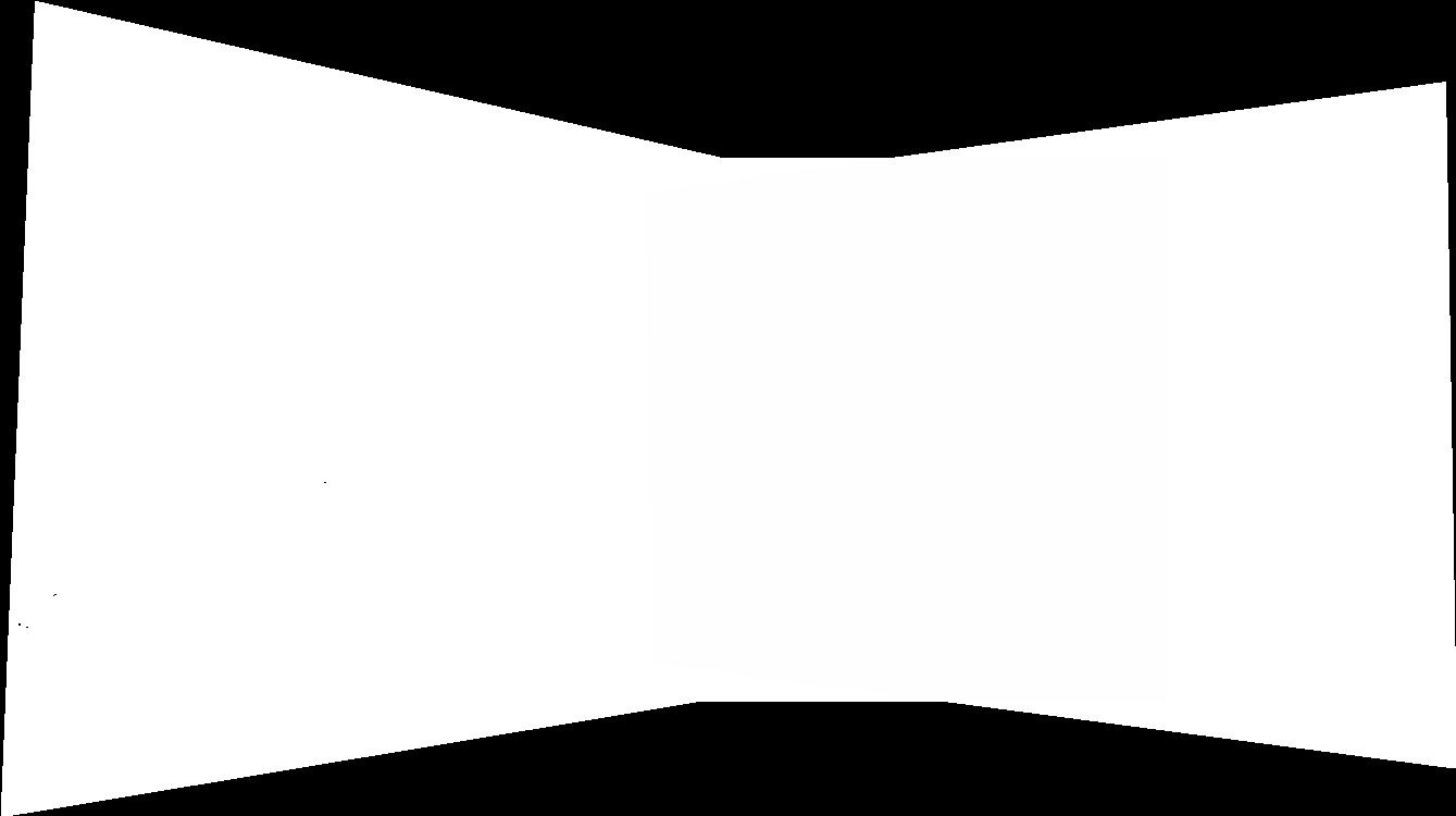
To blend the images together, I need to utilize bitmasks. I created bitmasks for my first and second images, as shown below, and "AND" them together to retrieve the overlapping bitmask. For all pixels that fall into this overlapped region, I employed a weighted average between the first and second image pixels and put these in my final mosaic. For all other pixels outside of the overlap mask, I extract them from their respective images.
To blend together 3 images, I combined images together one by one to the reference middle image. I first combined the left and middle image bitmasks together, blending using a weighted sum over the overlap mask. Then, I took this left + middle blended bitmask and combined it with the right bitmask, and again blending its overlap with a weighted sum. And as stated above, I extract all pixels outside of the overlap mask from their respective images.
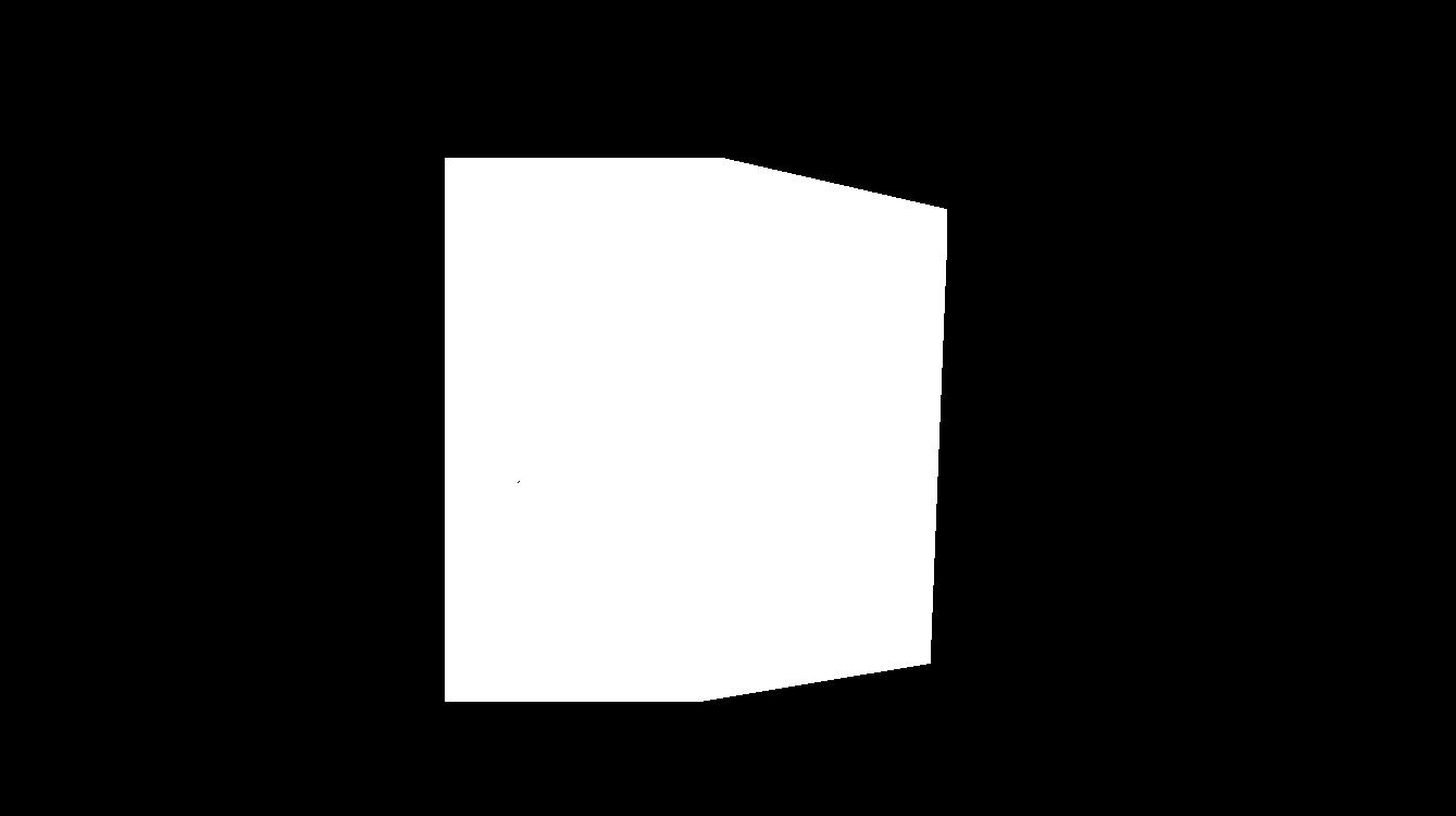
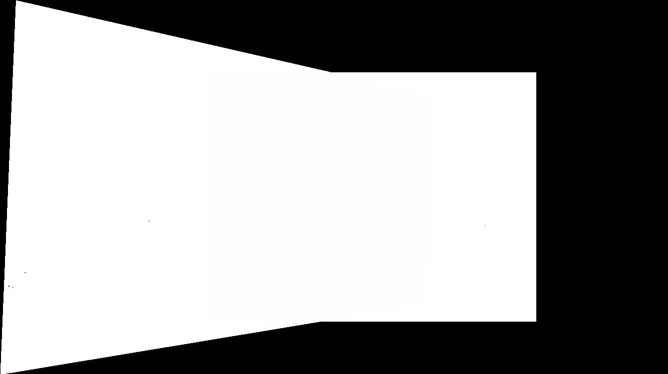

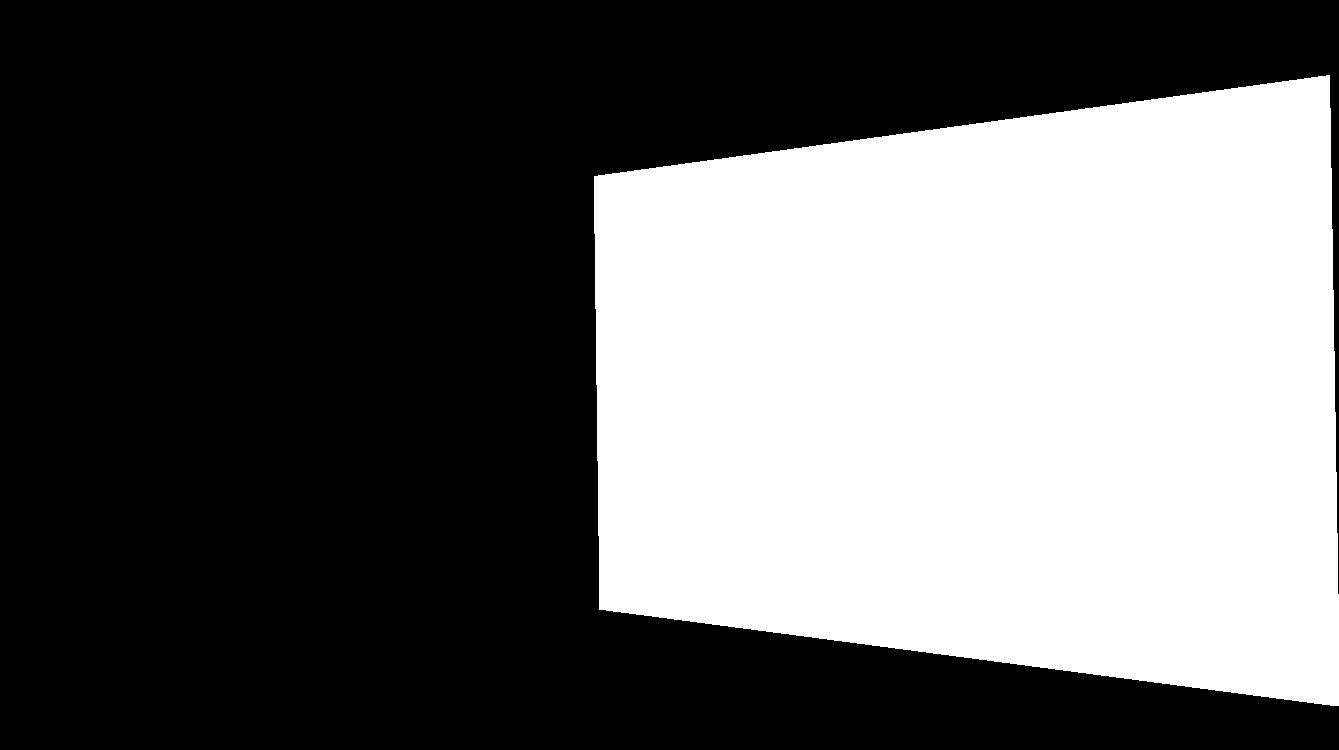
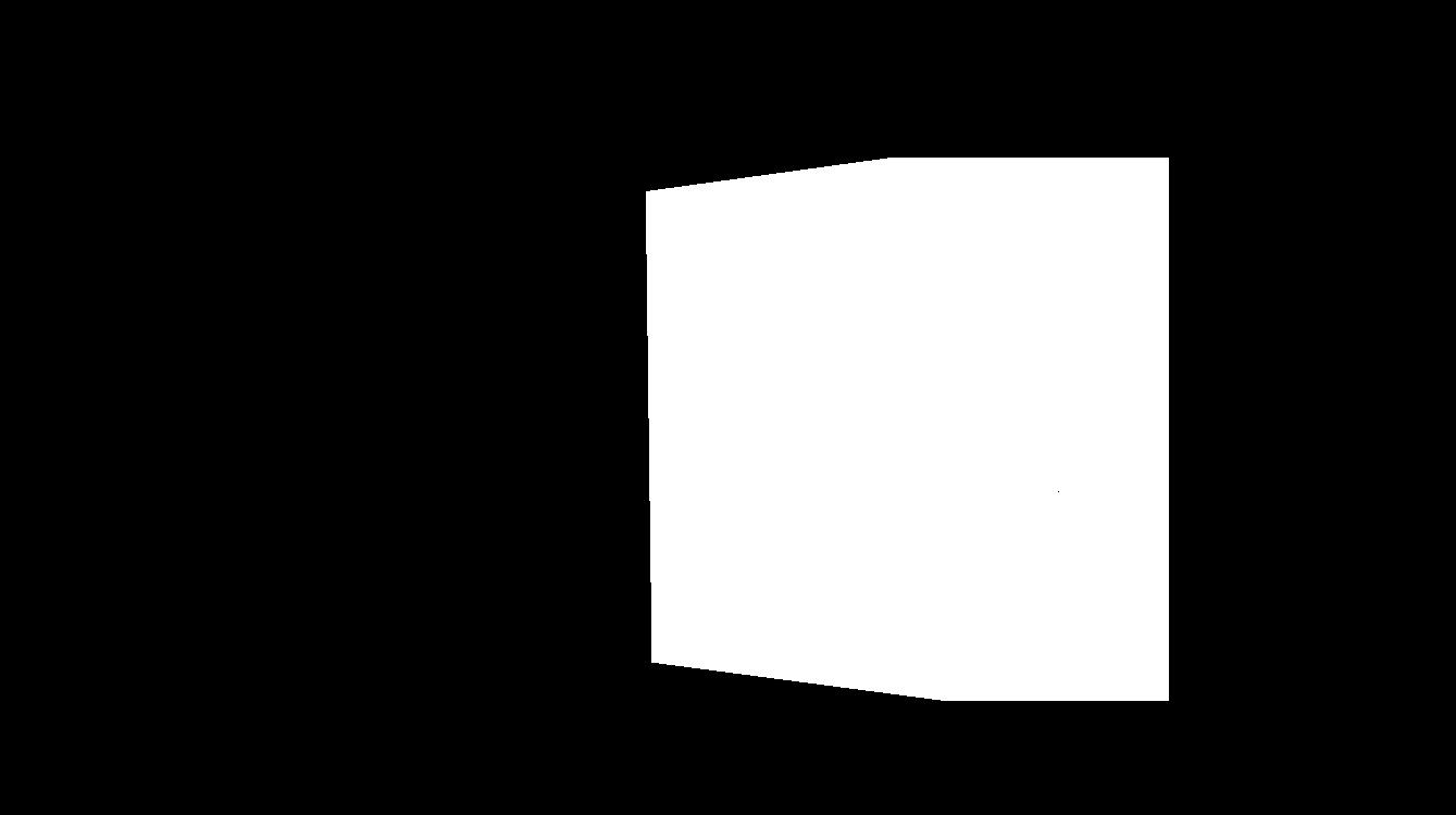
The final product is a combined panoramic mosaic of all 3 input images!

I repeated the same warping and bitmasking procedure as above, but this time leaving one of my images unwarped and warping the other image into its projection, producing two more mosaic images.




Part 4B
Part 2.1: Harris Point Detector
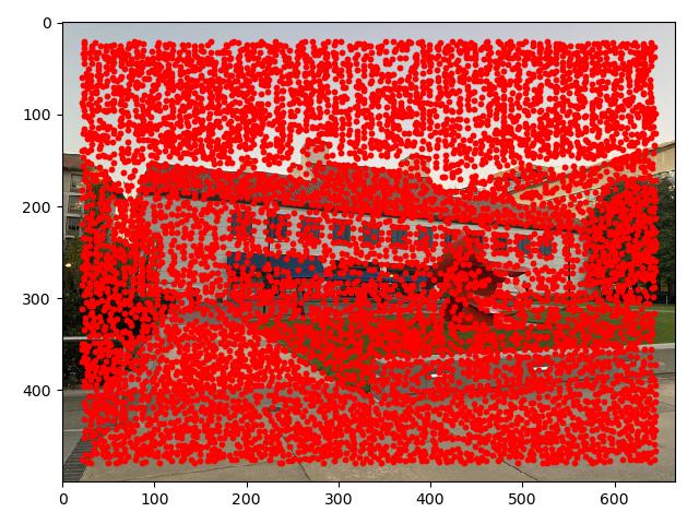
We first start by identifying the corners on our image, defined my by the Harris interest point detector. This corner detection is computed via gradients and then comparing its eigenvalues, and we pinpoint large and similar eigenvalues as those areas where a corner point is located. In other words, when you shift this area around in any way whatsoever, there will be some sort of change in the image.
Part 2.2: Adaptive Non-Maximimal Suppression
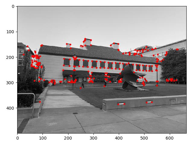
However, there are too many Harris corners to look at and we need to reduce these down to a more manageable sample. Rather than just selecting the points with the highest corner strength, we want to ensure our points are relatively evenly spaced out. To do this, we need to use adaptive non-maximal suppression (ANMS), which picks the top-K interest points such that its distance to the nearest interest point is significant larger. Essentially, within each neighborhood of radius r, we only maintain the maximum interest point within that region, and do this across our entire image such that our result will contain evenly distributed points throughout our image.
Part 2.3: Feature Description Extraction
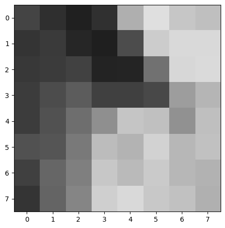
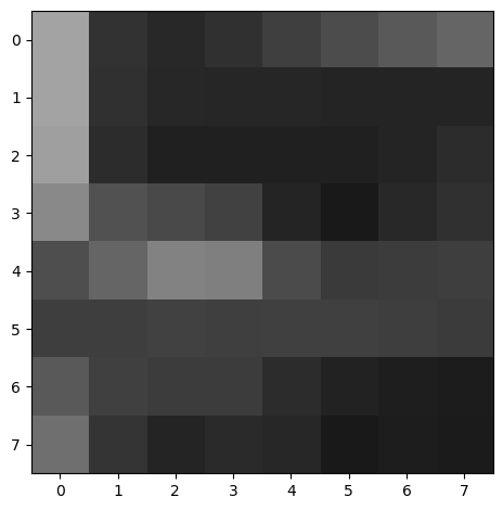
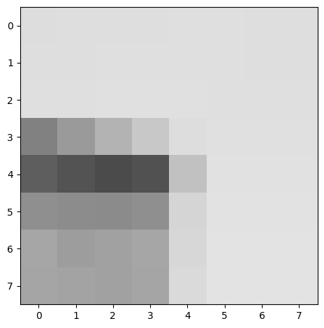
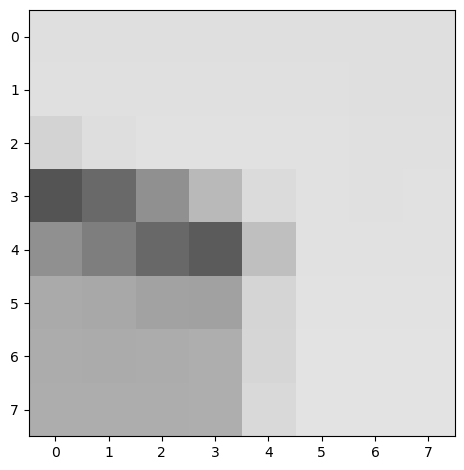
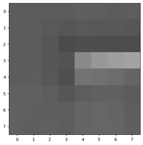
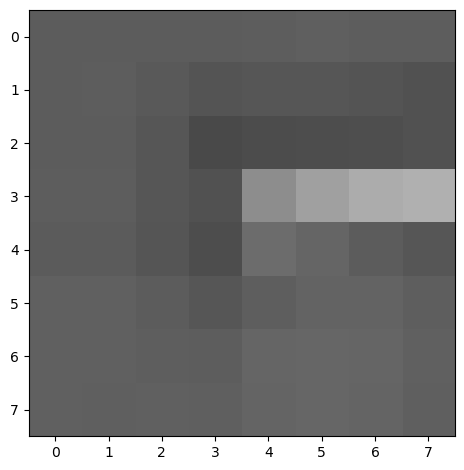
Once we've derived a solid set of ANMS points, we perform feature descriptor extraction. To do so, we compute a 40x40 axis-aligned patch centered around every interest point. Then, we blur it to ensure anti-aliasing, downscale it to 8x8, and then normalize using bias/gain. These feature descriptors will then later be used for comparison such that we can detect which points correspond to each other.
Below is an example of a couple of a feature descriptor we've extracted.
Part 2.4: Feature Matching
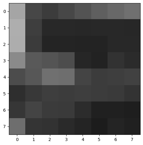
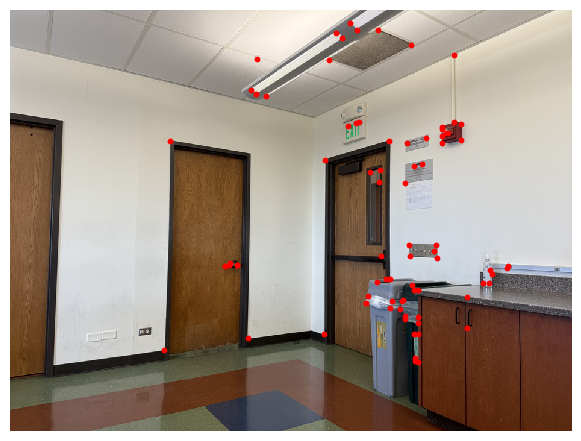
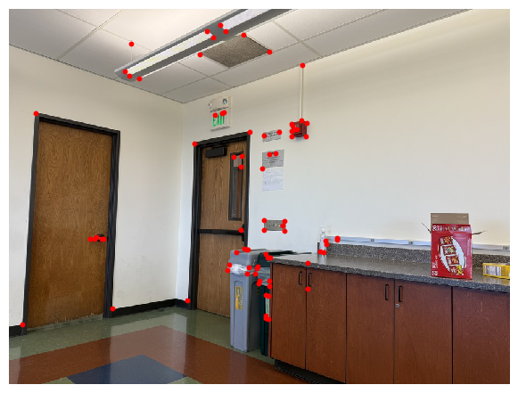
Equipped with our feature descriptors, now we need to decide which feature descriptors match each other. For each patch in the first image, we compare it to a patch in the second image by finding its sum-squared differences, then order them in ascending order of these differences. We decide which features to extract by calculating the ratio of the (first nearest neighbor error / second nearest neighbor error) and verifying if it's below a pre-determiend threshold, hence extracting only the feature descriptors that are similar enough.
Below are examples of feature descriptor matches we've computed between two separate images.
And here's the points feature matching managed to pinpoint:
Part 2.5: RANSAC
RANSAC, or random sample consensus, is a methodology utilized to estimate homographies by choosing correspondence points that best align together and discards outliers. With the points that we've sifted through feature matching, we can now use these points to compute our homography. Using a RANSAC loop, we select 4 of these feature pairs at random and compute its homography. Note, we don't have to use least squares when computing this homography because 4 feature pairs don't result in an overestimated system. Then, we calculate the Euclidean distance between these transformed points and our ground truth targets, and count and track the number of points whose distance is less than a pre-determined threshold--this is the number of inliners we have, and all other points above the threshold are our outliers which we ultimately filter out using this process. From there, we repeat this process for around 5000 steps and output the homography with the largest set of inliners.
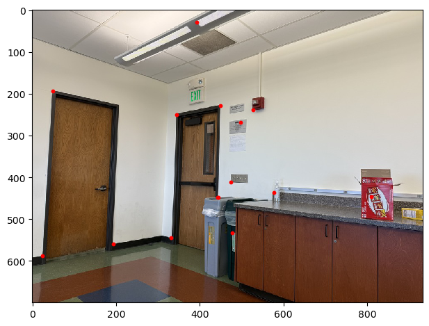
Let's walk through an example. Here, I have two images from earlier that I have computed already featured matched coordinates for from 500 harris corners.


I compute my inliners using the method described above, resulting in only the important points that correspond to each other. As you can see, all the extra points located near the outlet or the red box on the table are ignored, as these points don't match with any points in the other image, and hence we've filtered out these outliers.
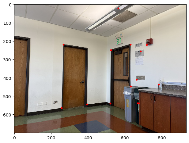
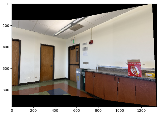
Finally, using these RANSAC points for each image, I compute and apply a homography to blend these two images together the same way I did in part A. And, voila! We have a beautifully blended mosaic of two images without having to manually select correspondence points.
Here's a couple of other blended pictures that have been autostitched together:
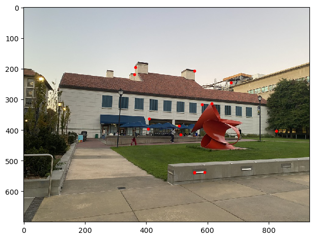
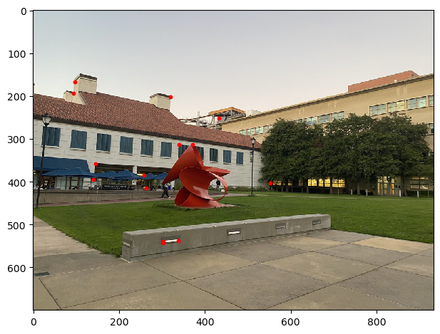
You can see a few discrepencies here. For example, I wasn't the most careful about the select of a couple of my manual points, causing the left-front tiles to not entirely match up. However, automatic stitching handled this more effectively and these tiles are better aligned.



Reflection
Overall, this project has taught me a lot about homographies and how image warping and alignment works. I think overall my results turned out relatively well because I took my pictures keeping the camera as steady as possible such that my center of projection was the same. Additionally, the image rectification proved my homography effective since my images were effectively made rectangular, and my final mosaics effectively blended my images together. I find automatic feature alignment to be so fascinating because of the careful computation behind it, and I think it reveals how cool and powerful the Gaussian is because it played a key role in feature matching. I also think RANSAC is a super cool method that feels brute force, but it is still so effective at being able to knock out outliers and consequently figure out what the homoegraphic transformation is supposed to look like.