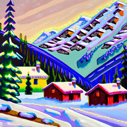
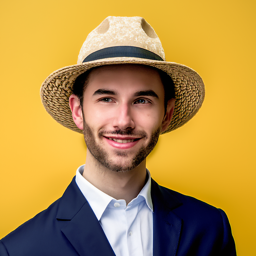
The random seed I used was 180. By providng text prompts and sampling from the model, I generated an image of an oil painting of a snow mountain village, a man wearing a hat, and a rocket ship using num_inference_steps = 20 and num_inference_steps = 70.

I added noise to an image via a forward process using equation 2.

I used the Gaussian blur filter to remove the noise from the noisy images generated in part 1.1.

Using the Unet, I estimate the noise by passing it through stage_1.unet and then subsequently remove this noise to estimate the original image in one step.

Rather than denoising in one step, I denoise starting from an i_start of 10 and iteratively across strided_timesteps starting at 990 and reducing by a stride of 30. Then I denoise using equation 3 every iteration.

To generate images from scratch, I utilize an i_start of 0 and pass in random noise to generate 5 high quality photos.

To improve image quality, we can employ classifier free guidance. This is done by computing both a conditional (condition on the text prompt) and an unconditional noise estimate (condition on null text prompt), and aggregating a new estimate from these two estimates that are scaled using a scale value of 7. These are the resulting high quality photos.

Here, we'll follow the SDEdit algorithm to make a series of edits that become more and more like our image using different starting indexes of 1, 3, 5, 7, 10, and 20.

Here, we're repeating the same SDEdit algorithm on images from the internet and handdrawn images.

Now, we want to isolate image generation and only run the diffusion denoising loop to within the bounds of a binary mask. Hence, I went ahead and created masks for my test, crater lake, and lantern images and impainted them.

Now, we're repeating the same SDEdit algorithm but using a text prompt. Using "a rocket ship" as our text prompt, this will transform our images more and more to look like a rocket ship.

Next, we want to create visual anagrams, which are images like look like one thing rightside up and look like something else upside down. To do this, we pass in two separate prompts, and denoise with each prompt. For the first prompt, we denoise as usual. For the second prompt, we flip the image upside first, compute the noise estimate, and then our noise estimate back to rightside up. We perform the reverse diffusion step using the average of these two noise estimates.

To create hybrid images we still use two separate prompts and generate noise estimates from them. Rather than flipped as in part 1.8, we run the first noise estimate through a low pass filter using a Gaussian kernel and the second noise estimate through a high pass filter (original - low pass). The combined low pass and high pass noise estimates are then used for the diffusion step.

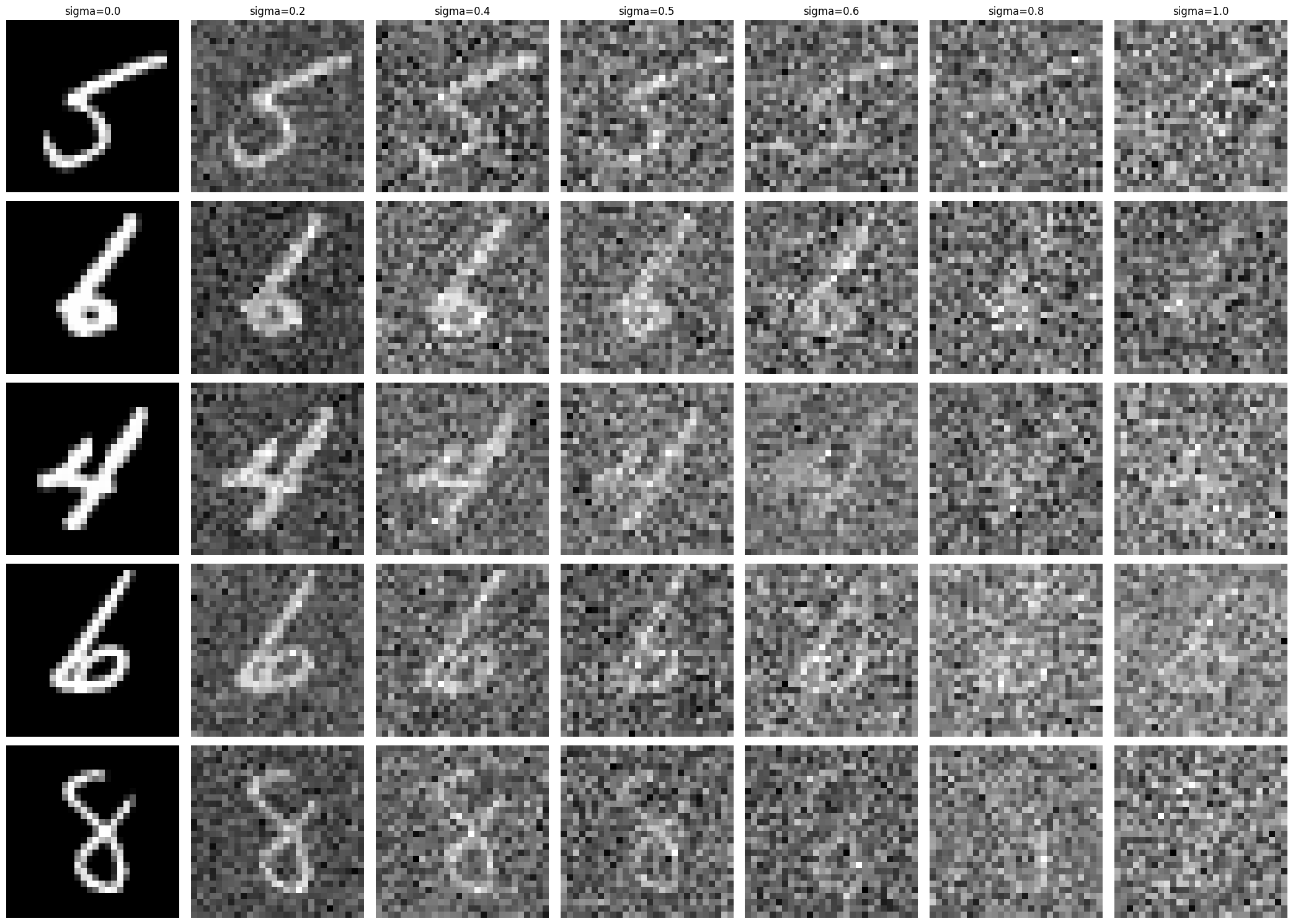
I constructing a denoiser as a UNEt by implementing its inner convolutional and average pooling layers and upscaling/downscaling/concatenating them as needed. I generated noisy images via z = x + sigma * epsilon and applied the denoiser to denoise the noisy images at varying sigma values. The result is shown in the figure below.

Then, I trained this denoiser optimized over L2 loss on the MNIST dataset.

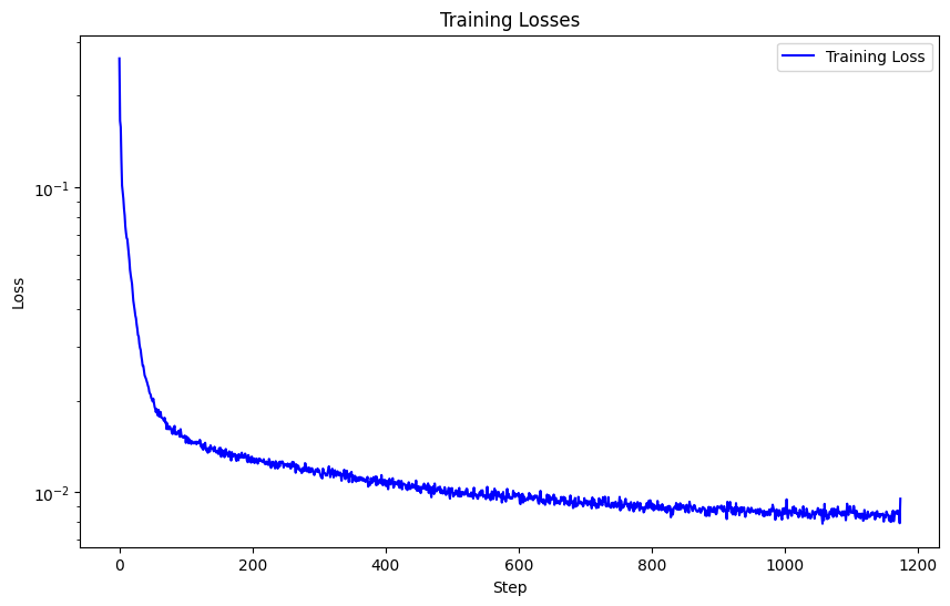
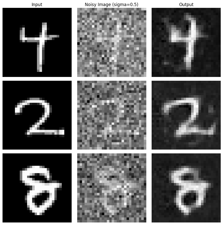
These are the denoised results on the test set after training on one epoch.

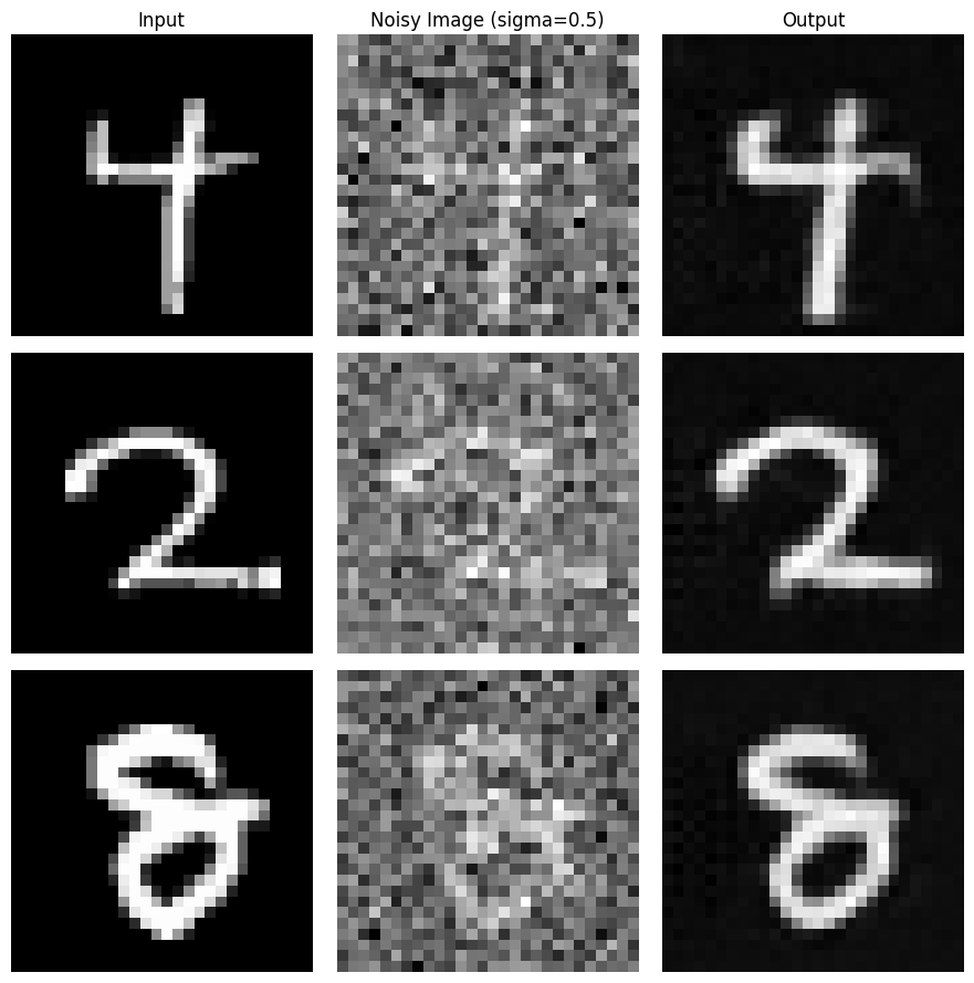
These are the denoised results on the test set after training on five epochs. As you can see, it performs better than one epoch.

Here is a visualization of denoising on varying levels of sigma.

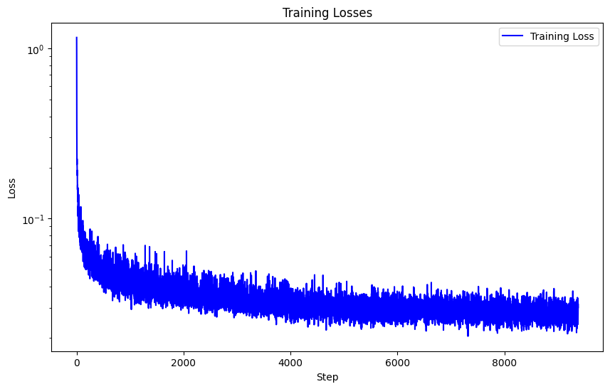
Next, I created a time-conditioned UNet that can iteratively denoise an image via DDPM. This is the loss associated with training 20 epochs on our new time-conditioned UNet.

These are the sampled results from the time-conditioned UNet for 5 and 20 epochs respectively.

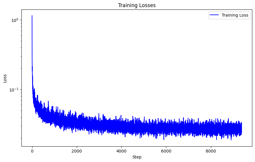
I also created a class-conditioned UNet that can iteratively denoise an image via DDPM with and without conditions This is the loss associated with training 20 epochs on our new time-conditioned UNet.

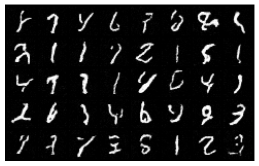
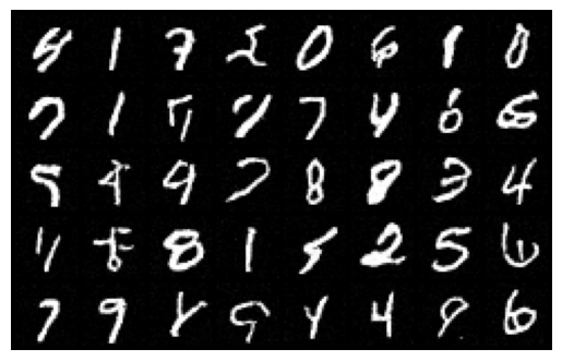
And these are the sampled results from the class-conditioned UNet for 5 and 20 epochs respectively.