Project 6: Final Project
Precanned 1: Gradient Domain
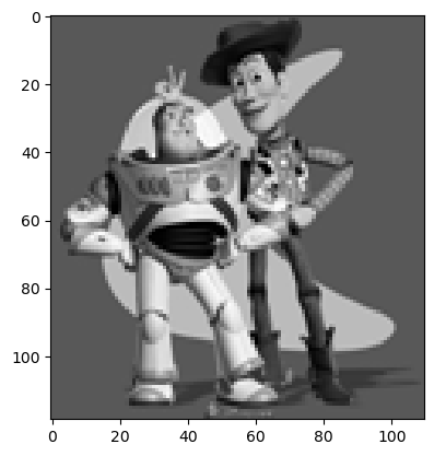
Part 2.1: Toy Problem
For the toy problem, we will reconstruct the toy image using its gradients and pixel intensities. Essentially, there are 3 objectives we are trying to fulfill:
- minimize ( v(x+1,y)-v(x,y) - (s(x+1,y)-s(x,y)) )^2
- minimize ( v(x,y+1)-v(x,y) - (s(x,y+1)-s(x,y)) )^2
- minimize (v(1,1)-s(1,1))^2

Part 2.2: Poisson Blending
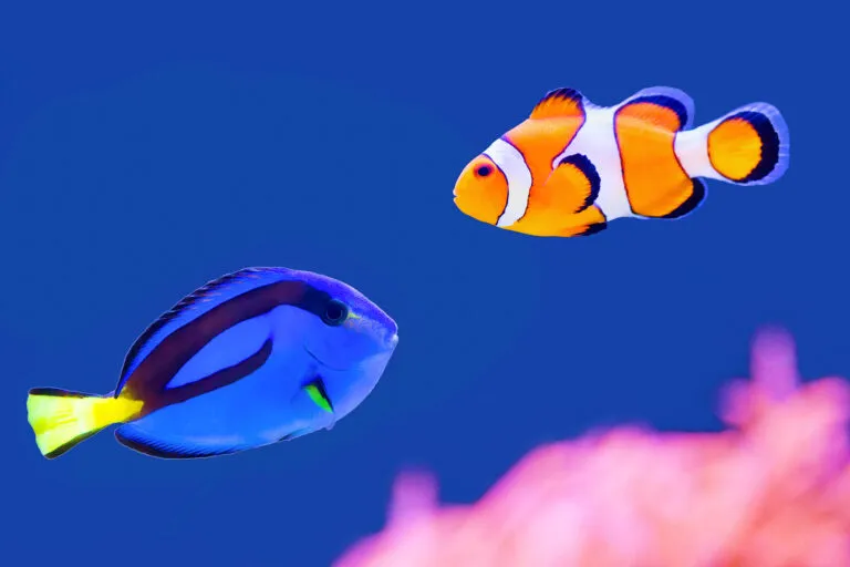
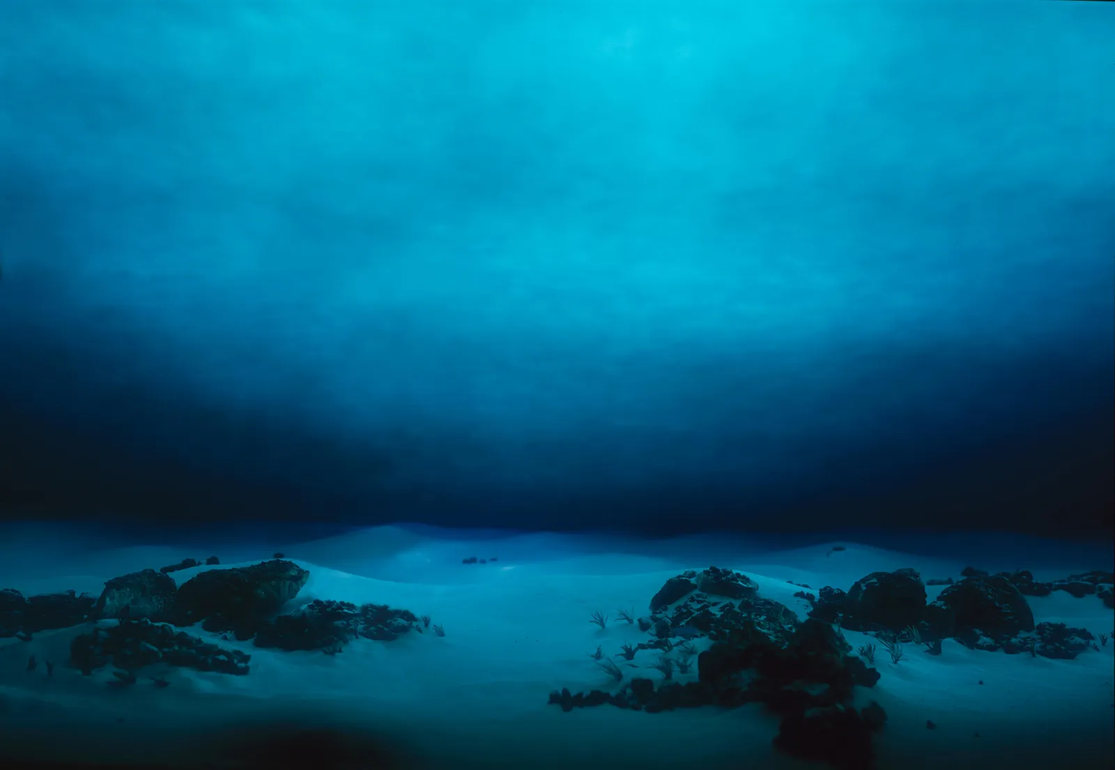
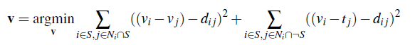
In poisson blending, the goal is to take a cutout of some source image and seamlessly paste it into a target image, blending the edges and ensuring similar gradients. To do this, we want to fulfill the following constraint below. Let S be the cutout region of our source image (in the dimensions of the target image) and let N be the four neighbors below, above, right, and left of the current pixel i.

Algorithmically, we are looping through our pixels and computing their pixel values depending on which case they fall under. Pixels will either:
- Reside outside of S
- Reside inside of S, and its neighbor also resides inside of S
- Reside inside of S, but its neighbor resides outside of S
For the second and third cases when we are looping over pixels that are in S, we want to check if its neighbors are also in S or not. If the neighbors are also in S, this alludes to the first half of the above constraint, which minimizes the difference between the values of this equation: v(x,y)-v(x_n,y_n) = s(x,y)-s(x_n,y_n). For the second half of the above constraint, we are dealing with pixels that are in S but its neighbors are outside of S, we directly use the target intensity of our neighbor (t_j) in our computation to minimize the values of this equation: v(x,y)-t(x_n,y_n) = s(x,y)-s(x_n,y_n).
Then, we solve this least squares problems where A is a matrix of (h * w, h * w) and b is a vector of length h * w. We do this for each of the rgb channels individually and then combining them together, we have a seamless poisson blended result.
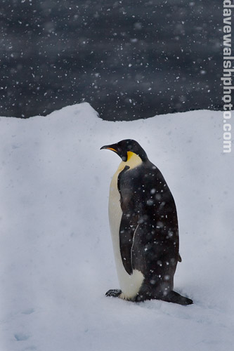
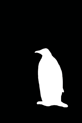
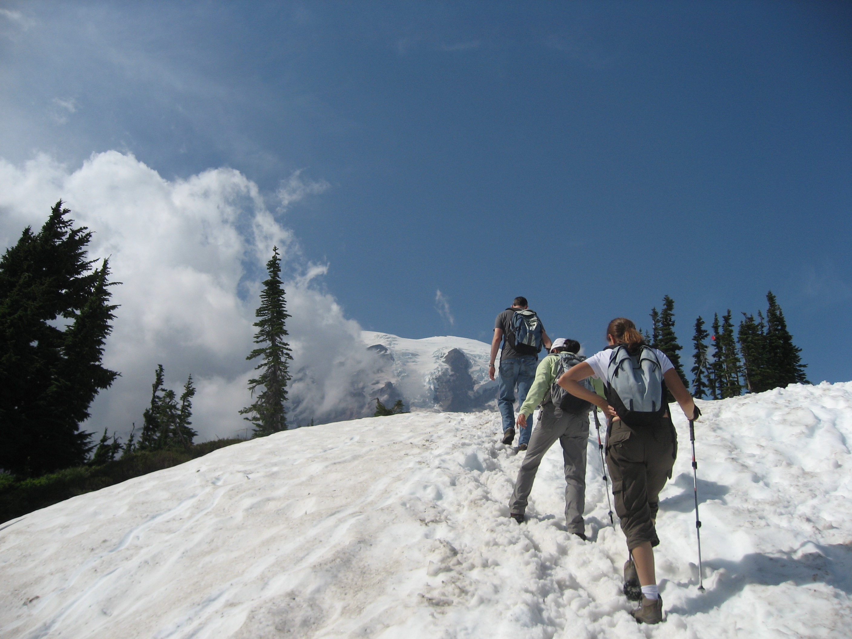

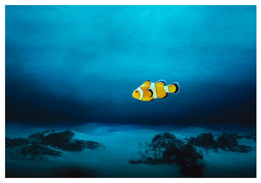
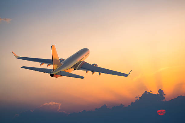
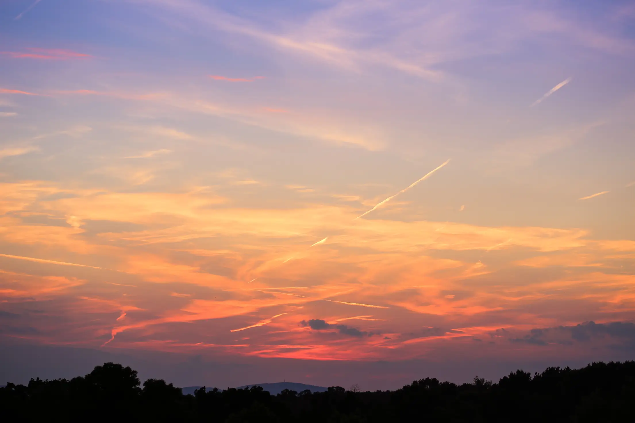
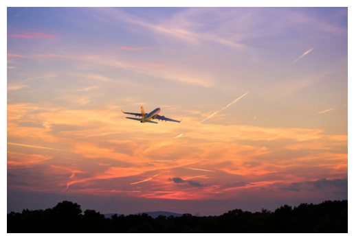
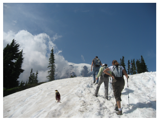
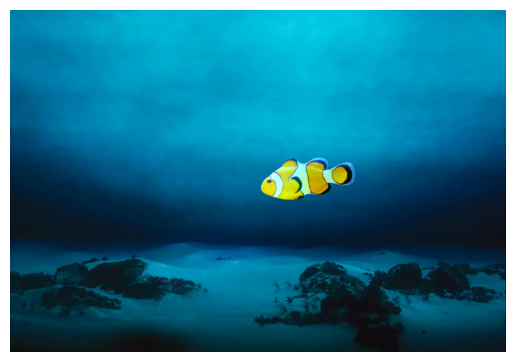
Each blended image also requires an offset variable bg_ul that we use to decide where in the background the object will be placed. The penguin I placed at (700, 400), the fish at (200, 200), and the plane at (250, 350). I noticed that my blends performed better when the background color matched the object itself. I also used more precise masks with a smaller border around the outside, and this resulted in darker outputs because there was less of the background in my masked image. But overall, the blends worked very well. Here are two more examples of poisson blending:


Bells & Whistles: Mixed Gradients
For mixed gradients, we want to similarly perform poisson blending but with a modified constraint equation:
In this case, we are mixing the gradients between the source and target images. To do this, we can take the absolute value of the source gradients, compare them against the absolute value of the target gradients, and take the larger of the two. In the above equation, d_ij corresponds to the larger gradient. Below are our results using mixed gradients compared to regular poisson blending. As you can see, the results tend to more closely match the background and hence are a little lighter.

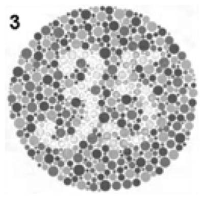
Bells & Whistles: Color2Gray
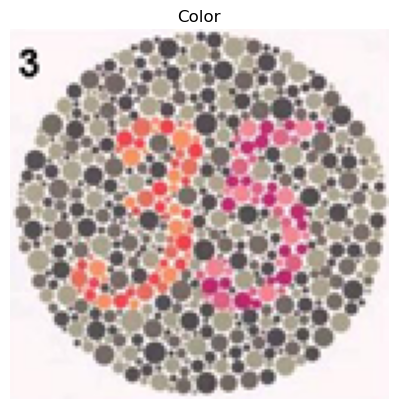
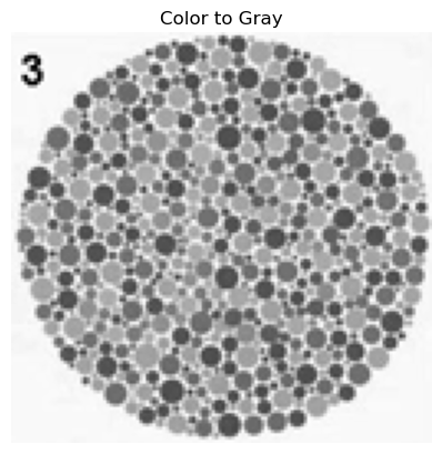
Normally when reconstructing an image, we convert it from color to grayscale using cv2.cvtColor(image, cv2.COLOR_BGR2GRAY). However, for images such as color blindness tests, converting these images to grayscale will cause them to lose their contrast and information.
To resolve this, we can try converting the image to the HSV space:
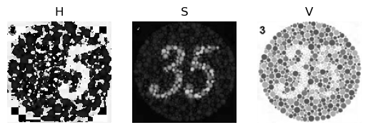
By using the V channel, which still preserves the information and intensities from the original image and properly converts it to grayscale, we're able to reconstruct the image properly with a MSE of 4.882742657242126e-13.
Precanned 2: Lightfield Camera
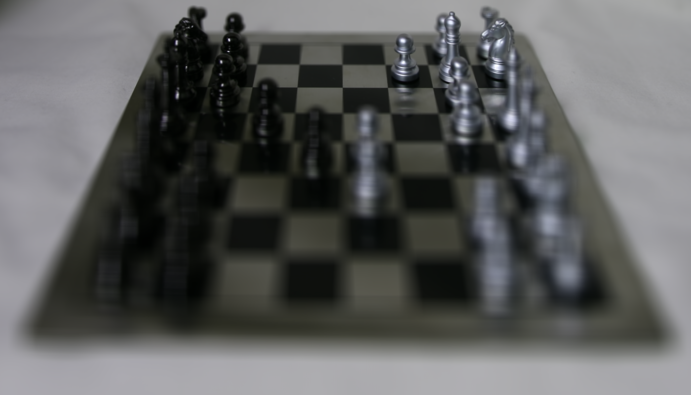
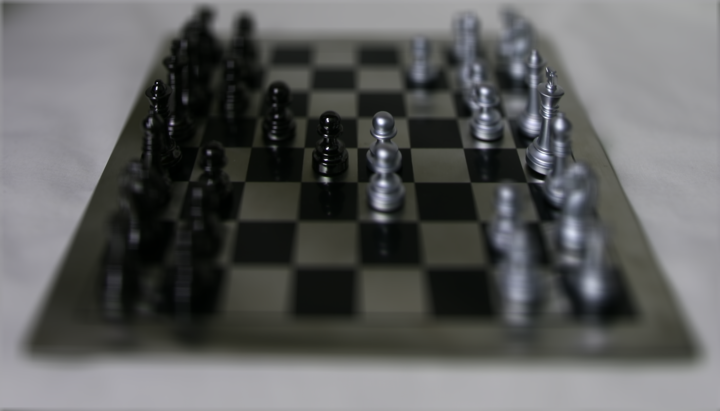
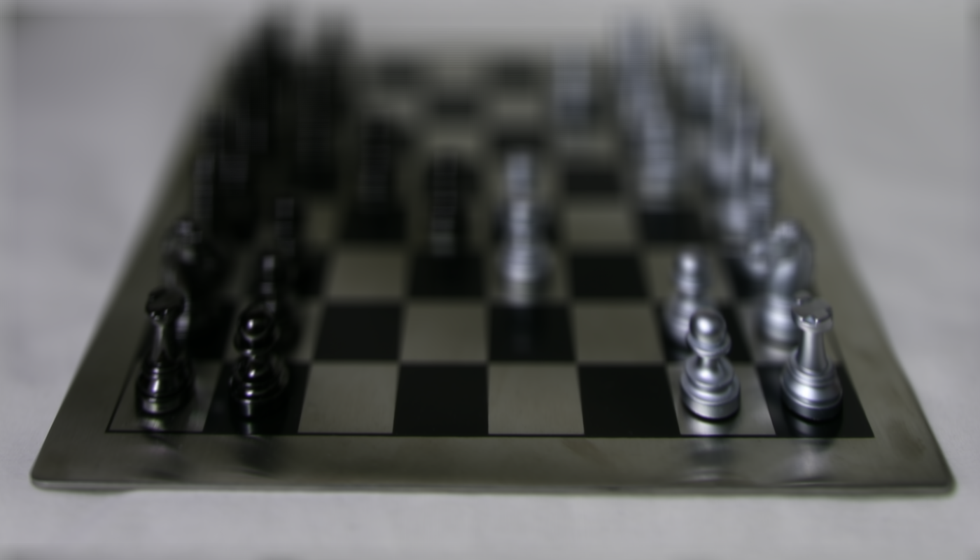
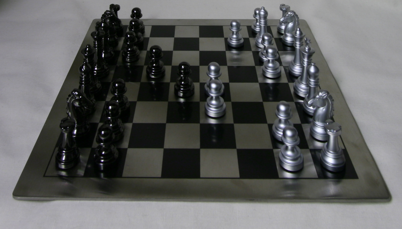
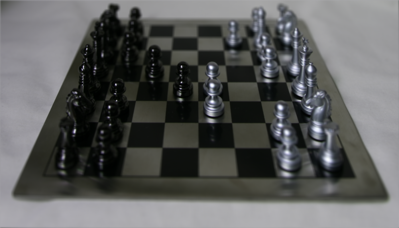
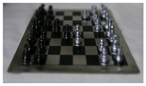
Part 1: Depth Refocusing
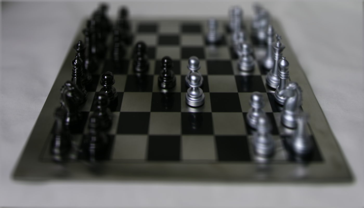
Using a series of rectified images of a chess board, a regularly spaced grid, I can refocus the depth of the image by reshifting. Typically, just averaging together all the images in the grid will cause blurriness in the front and sharpness in the back due to the large positional differences of nearby objects as opposed to faraway objects. However, we're able to specify areas of sharpness by shifting the images using np.roll appropriately. By using different depth_factor values, we're able to choose how close to the camera the sharpness is.
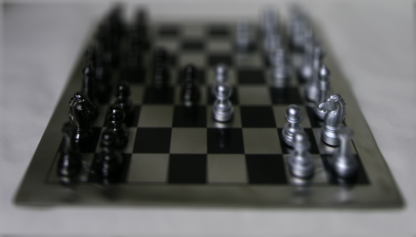
Part 2: Aperture Adjustment
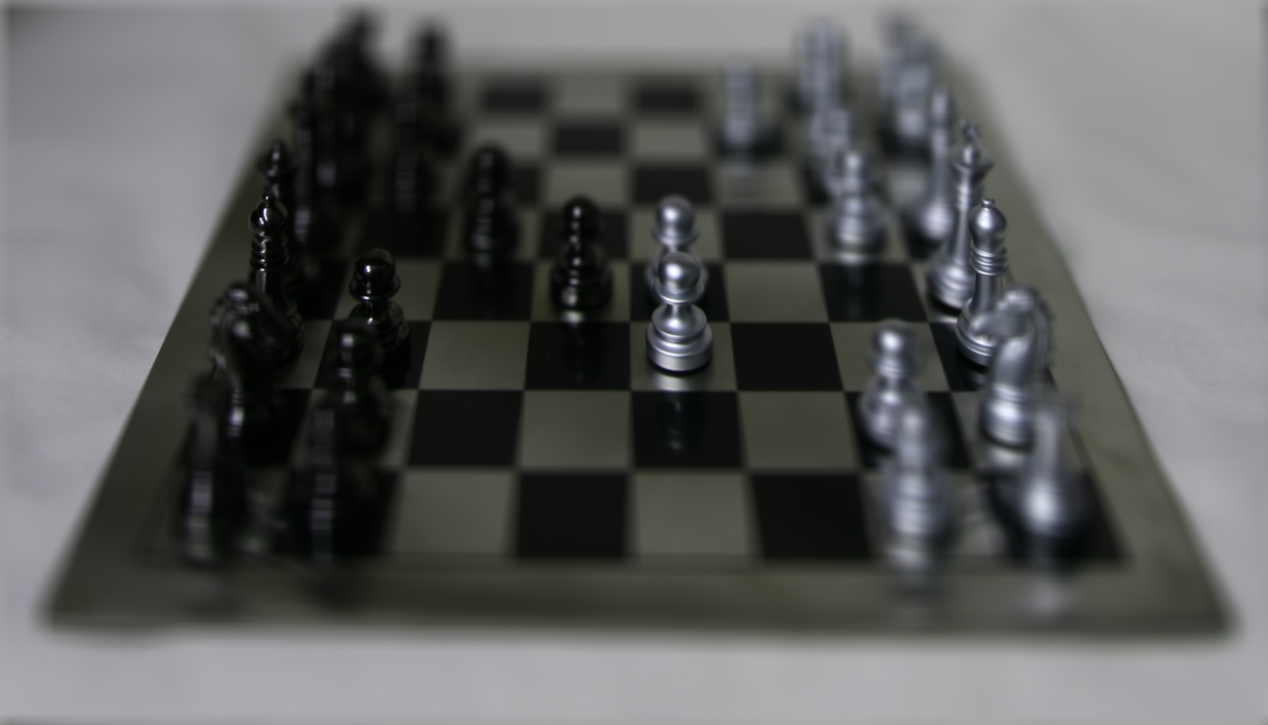
We're able to mimic variations in aperture by averaging over a different number of images. Modifying my refocus function by introducing an aperture parameter, I choose a smaller subset of images close to the center for a smaller aperture that still focuses on the same point, and vice versa. The results are shown below.
Summary
I am fascinated by how, just using images of a regularly spaced grid, we are able to change the visualization of the object in ways analogous to settings on a camera, including depth and aperture. These refocusing techniques only required averaging and shifting various images together and demonstrates how powerful lightfield data is.
Bells & Whistles: Interactive Refocusing
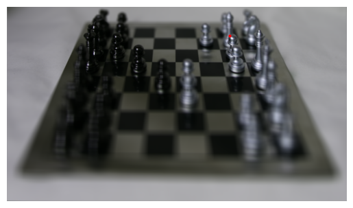
For interactive refocusing, we want to grant the user the ability to select an input point and make optimal pixel shifts such that the image is focused in a patch around the selected point. We can select for the point using plt.ginput. By selecting for a reasonable aperture, we optimize shifts for the depth_factor. Each selected point is displayed in red and the refocused results are shown below.

Bells & Whistles: NeRF Part 1
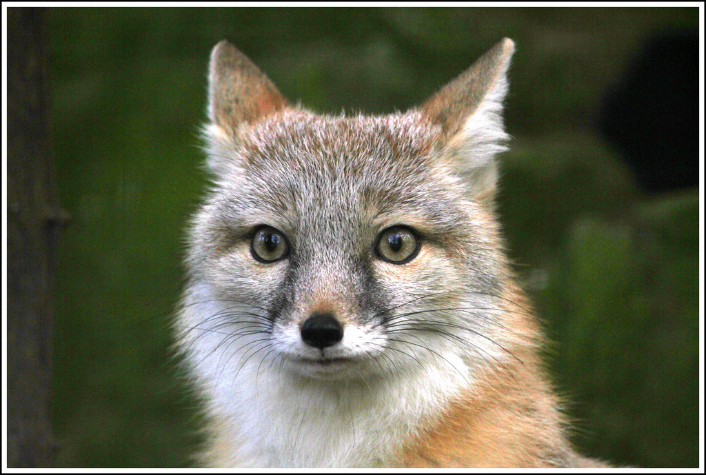
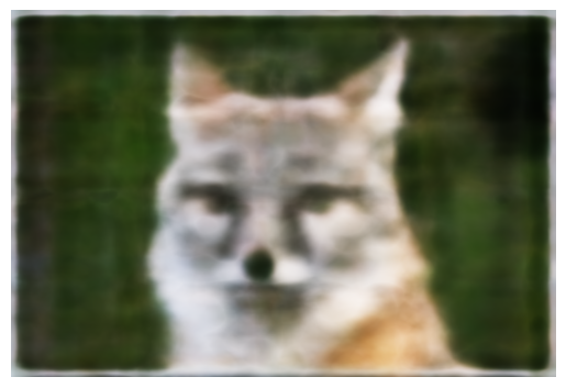
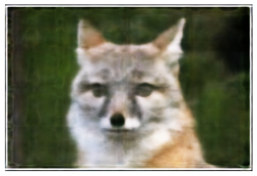
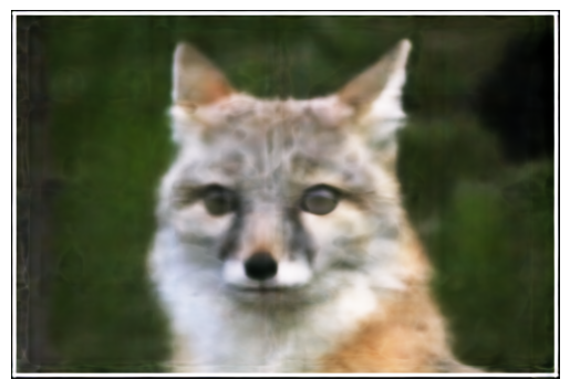
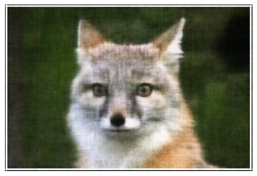
Neural radiance fields (NeRF) are used to map {x, y, z, θ, φ} to {r, g, b, σ}, or in other words, maps positionality and direction to color. In 2D, however, we map pixel coordinates (u, v) to {r, g, b} values. Here is an image of a fox we will use to apply NeRF to.
The architecture of my model is as follows:
First, I randomly sampled N = 1000 pixels for training, giving me 1000 x 2 2D coordinates as well as their
respective colors which have coordinates 1000 x 3 for the rgb channels. These are normalized and converted
into tensors in the random_sample_pixels method. Then, I implemented sinusoidal positional encoding (PE) to
expand the dimensionality of my randomly sampled input coordinates from 2D to a 42 dimension vector. Finally,
to build my MLP model, I chained together a series of nonlinear activations between layers, which includes 3 ReLU
opreations and then a sigmoid to clamp the values. The input dimensions I specify as 42 (which is the output of PE) and my final
output dimensions is 3, because I am outputing 3 dimensions of rgb to get a valid pixel color.
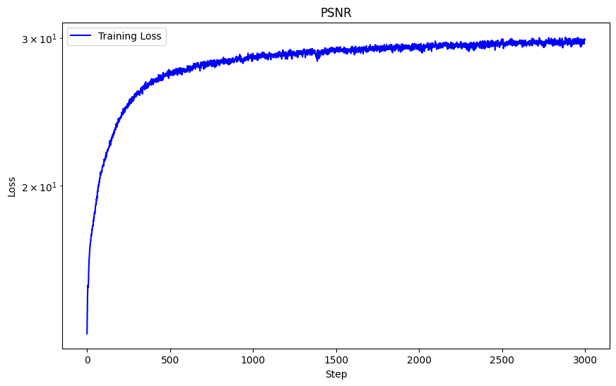
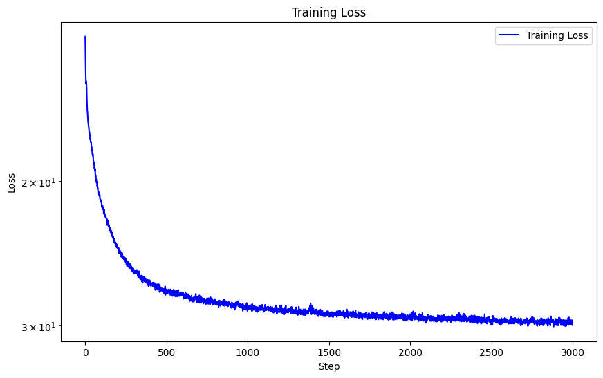
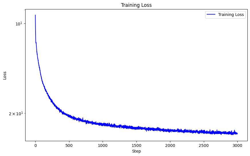
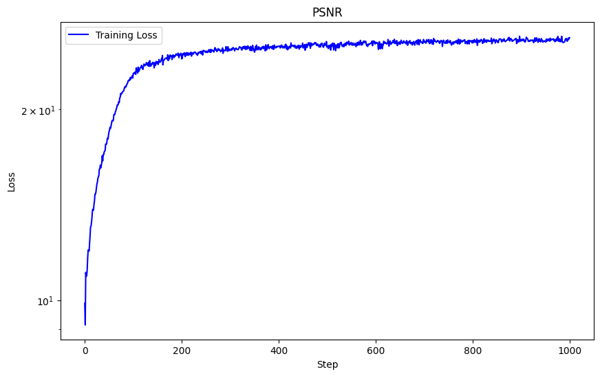
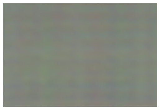
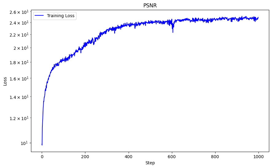
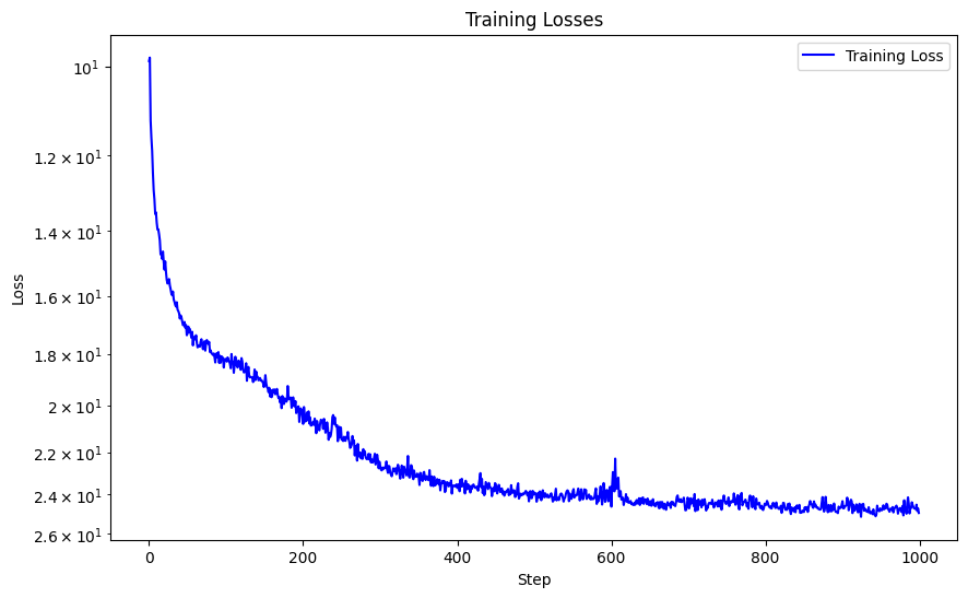
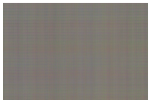
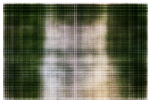
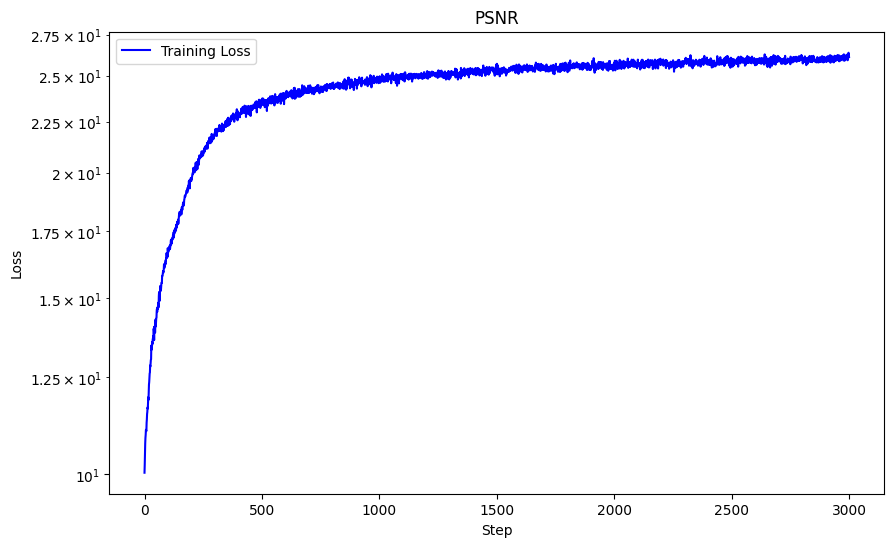
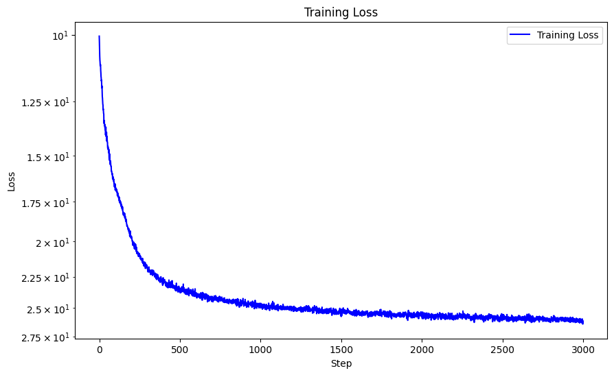
Below is a visualization of the training process of the predicted images across iterations with L = 10 (highest
frequency level), MSE loss function, Adam optimizer with learning rate 1e-2, batch size 10,000, trained over 3000 iterations.
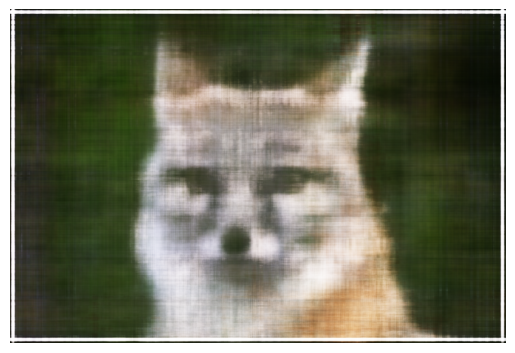
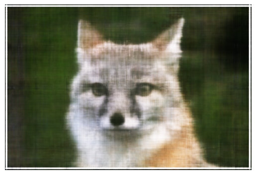
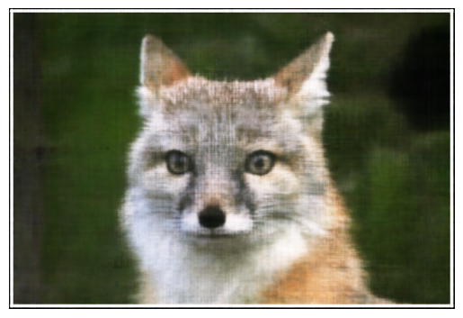
Here are the side-by-side results.
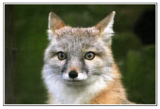
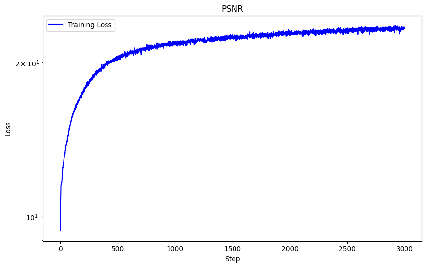
With these hyperparameters, I achieved a PSNR of 25.96.
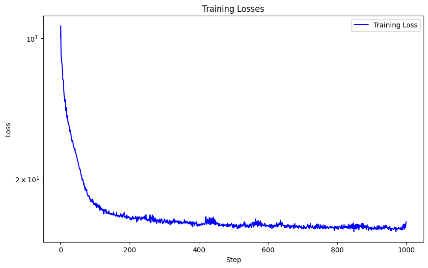
One hyperparameter I modified was the max frequency L for positional encoding, and instead of 10 I used L = 5. We can see the striations are not as thin and the overal picture is blurrier. This caused the sharpness in detail to significantly decrease due to the usage of lower frequency components, and hence diminished the performance of my network. With this hyperparameter modification, I achieved a lower PSNR of 24.92.
I also attempted to modify the learning rate to see how this would affect my network. By using a learning rate of 1e-3 instead of 1e-2. This yielded slightly better results with a PSNR of 26.12 and its curve is also much more stable. The details are slightly sharper than using a learning rate of 1e-2. For example, the hairs on the top of the fox are more defined and there is more contrast than in 1e-3 than 1e-2.


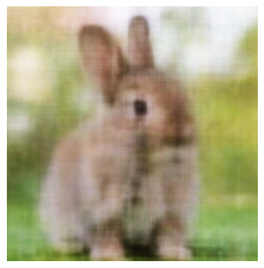
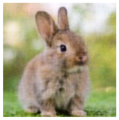
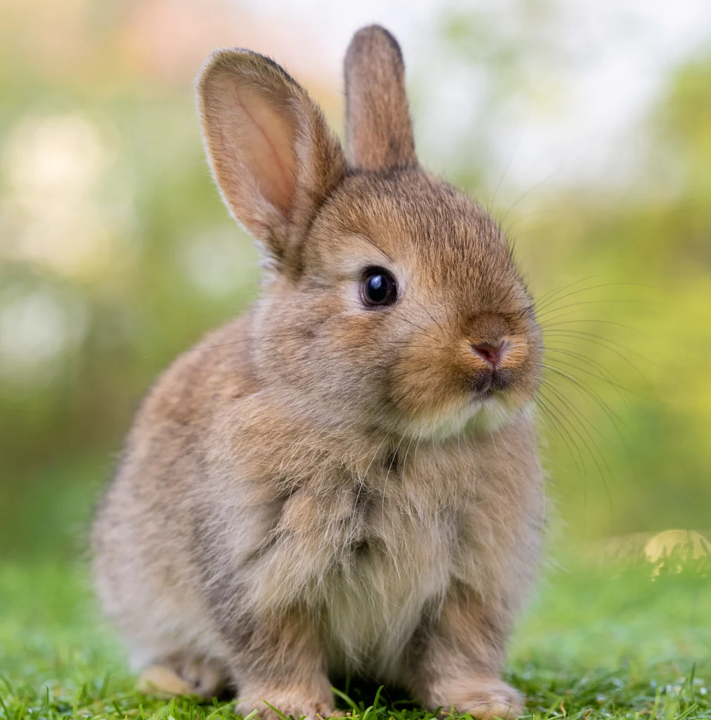
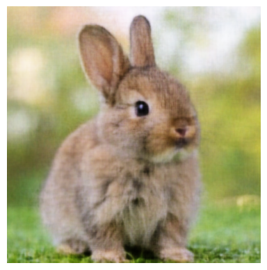
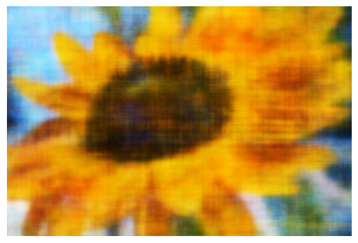
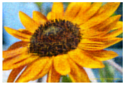
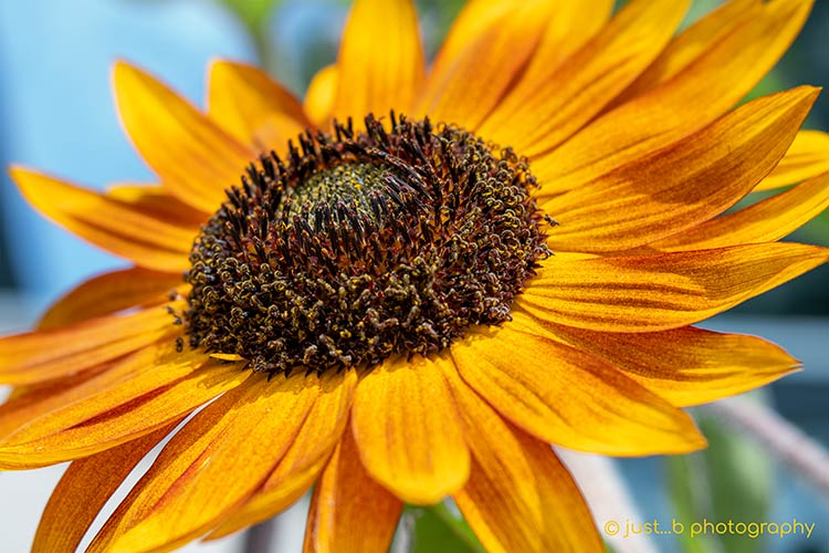
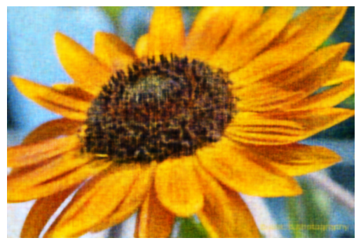
Here I run the model with these hyperparameters against two different images of my own choosing: L = 10, MSE loss function, Adam optimizer with learning rate 1e-3, batch size 10,000, trained over 3000 iterations. The bunny computed with PSNR = 29.90 and the sunflower computed with PSNR = 23.43.